1. Catalyst screening with a linear mixed model

This tutorial ranks catalyst candidates while accounting for measurements that share a synthesis or reactor batch. It is the materials-discovery counterpart to a blocked experiment: candidate identity and temperature are the effects of scientific interest, while the batch intercept represents shared conditions that are difficult to reproduce exactly.

Download the executed notebook

1.1. What you will learn

By the end of the analysis, you will be able to:

• build a deterministic, balanced catalyst-screening dataset;

• distinguish candidate and temperature fixed effects from a batch random intercept;

• explain and compile a model before optimization;

• fit a Gaussian linear mixed model (LMM) with restricted maximum likelihood (REML);

• inspect structured convergence, fixed-effect uncertainty, predictions, residuals, and provenance; and

• translate model output into a candidate ranking without treating that ranking as an automated discovery decision.

1.2. Domain question

Five candidates are tested in 12 batches. Every batch contains every candidate at two temperatures, which prevents candidate identity from being confounded with temperature. The response is product yield in percent.

The fitted model is

\[ y_{ij} = \beta_0 + \beta_{\text{candidate}(i)} + \beta_T(T_{ij}-320) + b_j + \epsilon_{ij}, \]

where \(b_j\) is a batch-specific random intercept. Centering temperature at 320 °C makes the intercept and adjusted candidate means directly interpretable at a useful operating point.

1.3. Dataset snapshot

Property	Value
Analysis rows	120
Batches	12
Candidates	5
Runs per batch	10
Nominal temperatures	310 and 330 °C
Response	Product yield (%)
Generating batch SD	2.2 percentage points
Generating measurement SD	1.4 percentage points
Random seed	20260723

The committed raw mean yields are 58.6892% for Cat-A, 61.5274% for Cat-B, 57.0792% for Cat-C, 63.5104% for Cat-D, and 60.0462% for Cat-E. These are descriptive checks only; they do not adjust for temperature or batch.

1.4. Reproduce the data

The following excerpts are the runnable core of the executed notebook. Run them in order.

import importlib
import logging
from pprint import pprint

import numpy as np

import pymixef

# Keep first-run Matplotlib font-cache status out of committed showcase output.
logging.getLogger("matplotlib.font_manager").setLevel(logging.ERROR)
plt = importlib.import_module("matplotlib.pyplot")

print("PyMixEF version:", pymixef.__version__)

plt.rcParams.update(
    {
        "figure.dpi": 110,
        "font.size": 10,
        "axes.titleweight": "semibold",
    }
)

rng = np.random.default_rng(20260723)

candidate_levels = np.array(["Cat-A", "Cat-B", "Cat-C", "Cat-D", "Cat-E"])
n_batches = 12
runs_per_batch = len(candidate_levels) * 2

candidate = np.tile(np.repeat(candidate_levels, 2), n_batches)
batch = np.repeat(
    [f"batch-{index + 1:02d}" for index in range(n_batches)],
    runs_per_batch,
)
nominal_temperature = np.tile(
    np.tile([310.0, 330.0], len(candidate_levels)),
    n_batches,
)
temperature_c = nominal_temperature + rng.normal(0.0, 1.0, candidate.size)
temperature_centered = temperature_c - 320.0

true_candidate_effect = {
    "Cat-A": 0.0,
    "Cat-B": 3.0,
    "Cat-C": -1.5,
    "Cat-D": 5.5,
    "Cat-E": 1.8,
}
batch_effect = rng.normal(0.0, 2.2, n_batches)
yield_pct = np.array(
    [
        58.0
        + true_candidate_effect[name]
        + 0.12 * centered_temperature
        + batch_effect[row // runs_per_batch]
        + rng.normal(0.0, 1.4)
        for row, (name, centered_temperature) in enumerate(
            zip(candidate, temperature_centered, strict=True)
        )
    ]
)

screening_data = {
    "yield_pct": yield_pct,
    "candidate": candidate,
    "temperature_centered": temperature_centered,
    "batch": batch,
}

1.5. Step 1: declare and explain the model

candidate and temperature_centered are fixed effects. (1 | batch) introduces one shared offset per batch and the distribution that connects those offsets. PyMixEF sorts string factor levels deterministically, so Cat-A is the reference candidate.

lmm_model = pymixef.Model.from_formula(
    "yield_pct ~ candidate + temperature_centered + (1 | batch)"
)

print(lmm_model.explain(screening_data, engine="lmm", method="reml"))

The dry explanation reports an \(X\) matrix with 120 rows, six columns, and rank six. It also reports one random-effect block with 12 batch groups and no excluded rows.

1.6. Step 2: compile and audit

Compilation resolves formula semantics, factor coding, row inclusion, compatibility, and ModelIR before any optimizer runs.

lmm_plan = lmm_model.compile(
    screening_data,
    engine="lmm",
    method="reml",
)

print(lmm_plan.explain())
print("\nAnalysis rows:", lmm_plan.matrices.audit.analysis_rows)
print("Excluded rows:", lmm_plan.matrices.audit.excluded_rows)
print("Factor levels:", dict(lmm_plan.matrices.factor_levels))

The committed audit retains all 120 source rows and archives the factor order ('Cat-A', 'Cat-B', 'Cat-C', 'Cat-D', 'Cat-E').

1.7. Step 3: fit and check convergence

lmm_fit = lmm_plan.fit()
print(lmm_fit.summary())

Interpret coefficients only after checking the structured convergence report.

convergence = lmm_fit.convergence
pprint(
    {
        "status": convergence.status,
        "trustworthy": convergence.trustworthy,
        "optimizer_terminated": convergence.optimizer_terminated,
        "iterations": convergence.iterations,
        "scaled_gradient_inf_norm": convergence.scaled_gradient_inf_norm,
        "hessian_positive_definite": convergence.hessian.positive_definite,
        "warning_codes": [warning.code for warning in convergence.warnings],
    }
)

assert convergence.trustworthy, "Review convergence before interpretation."

The saved fit is trustworthy, has a positive-definite Hessian, contains no warning codes, and has a scaled-gradient infinity norm of 5.684341889072788e-06.

1.8. Step 4: inspect estimates and uncertainty

Candidate coefficients are adjusted differences from Cat-A at 320 °C. The temperature coefficient is the expected change in yield for one additional degree Celsius. The batch and residual standard deviations describe heterogeneity, not candidate effects.

fixed_names = list(lmm_fit.extra["fixed_effect_names"])
fixed_covariance = np.asarray(lmm_fit.extra["fixed_effect_covariance"])
fixed_standard_errors = np.sqrt(np.diag(fixed_covariance))

print(f"{'fixed effect':32s} {'estimate':>12s} {'std. error':>12s}")
for name, standard_error in zip(fixed_names, fixed_standard_errors, strict=True):
    print(f"{name:32s} {lmm_fit.parameters[name]:12.4f} {standard_error:12.4f}")

1.8.1. Key saved results

Quantity	Estimate	Standard error
Intercept	58.6840	0.4361
Cat-B minus Cat-A	2.8514	0.3662
Cat-C minus Cat-A	-1.6117	0.3662
Cat-D minus Cat-A	4.8226	0.3662
Cat-E minus Cat-A	1.3998	0.3663
Temperature slope per °C	0.1070	0.0117
Batch-intercept SD	1.2157	—
Residual SD	1.2687	—
Objective	214.2828458	—
Log likelihood	-214.2828458	—

At 320 °C and a zero batch effect, the committed adjusted ranking is:

Rank	Candidate	Adjusted mean yield
1	Cat-D	63.51%
2	Cat-B	61.54%
3	Cat-E	60.08%
4	Cat-A	58.68%
5	Cat-C	57.07%

reference_mean = lmm_fit.parameters["Intercept"]
adjusted_candidate_mean = {}
for name in candidate_levels:
    coefficient_name = f"candidate[{name}]"
    adjusted_candidate_mean[name] = reference_mean + lmm_fit.parameters.get(
        coefficient_name, 0.0
    )

ranking = sorted(
    adjusted_candidate_mean.items(),
    key=lambda item: item[1],
    reverse=True,
)
assert ranking[0][0] == "Cat-D", "The synthetic screen should rank Cat-D first."

1.9. Step 5: visualize adjusted performance

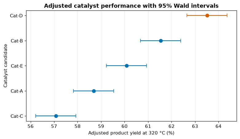
Adjusted catalyst performance with 95% Wald intervals. Candidate means are evaluated at 320 °C with the batch random effect set to zero.

Interpretation. Cat-D has the highest adjusted mean in this deterministic screen. The intervals communicate estimation precision, but a formal candidate comparison should be based on planned contrasts rather than rank alone.

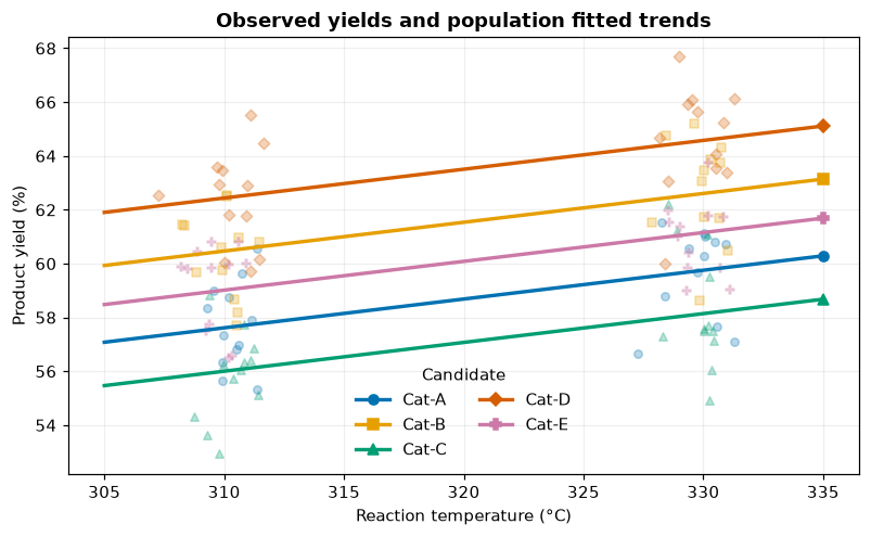
Observed yields and population fitted trends. Markers retain the experimental spread and lines show model-implied fixed-effect trends.

Interpretation. The fitted lines are parallel because the model contains one common temperature slope and no candidate-by-temperature interaction. The observed spread includes batch heterogeneity and measurement error represented elsewhere in the model.

1.10. Step 6: name the prediction target

Conditional predictions include estimated batch effects. Population predictions set the batch effect to zero.

conditional = lmm_fit.prediction(mode="conditional")
population = lmm_fit.prediction(mode="population")
observed = np.asarray(screening_data["yield_pct"])

conditional_rmse = float(np.sqrt(np.mean((observed - conditional) ** 2)))
population_rmse = float(np.sqrt(np.mean((observed - population) ** 2)))
assert conditional_rmse < population_rmse

residual_table = lmm_fit.residual_diagnostics()

The saved conditional RMSE is 1.182, compared with 1.698 for population predictions. That comparison is expected on the same fitted batches because conditional predictions use their estimated effects.

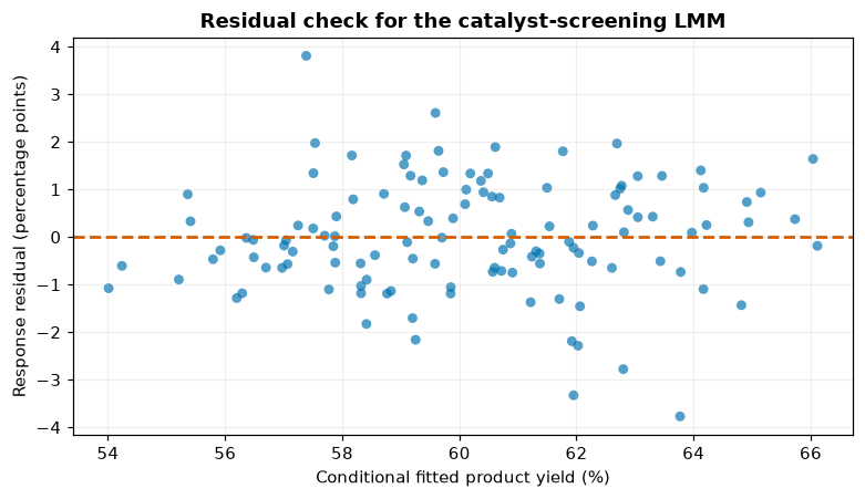
Residual check for the catalyst-screening LMM.

Interpretation. Residuals remain centered near zero without a strong curve or funnel in this synthetic realization. A real screen should add influence checks and prespecified sensitivity analyses.

1.11. Step 7: preserve provenance

manifest = lmm_fit.manifest.to_dict()
pprint(
    {
        key: manifest[key]
        for key in (
            "package_version",
            "engine",
            "method",
            "model_ir_hash",
            "data_hash",
            "reproducibility_class",
        )
    }
)

The saved result records a deterministic-with-tolerance reproducibility class, the model and data hashes, and the optimizer sequence L-BFGS-B → Powell rescue → L-BFGS-B refinement.

1.12. API map

Task	Public API
Declare the formula	pymixef.model.Model.from_formula()
Preview compatibility and matrices	pymixef.model.Model.explain()
Compile and audit	pymixef.model.Model.compile(), pymixef.model.ExecutionPlan.explain()
Fit	pymixef.model.ExecutionPlan.fit()
Read estimates	pymixef.results.FitResult.parameters
Read fixed-effect covariance	pymixef.results.FitResult.extra
Check convergence	pymixef.results.FitResult.convergence
Select a prediction target	pymixef.results.FitResult.prediction()
Build residual diagnostics	pymixef.results.FitResult.residual_diagnostics()
Inspect provenance	pymixef.results.FitResult.manifest, pymixef.provenance.RunManifest.to_dict()

Interpretation boundaries

This balanced synthetic screen is a compact way to learn the complete audited workflow. For a discovery decision, strengthen the same workflow with planned contrasts, candidate-by-temperature sensitivity, durability and selectivity measurements, explicit missing-data reasoning, physical characterization, and independent confirmation. Population predictions describe an average batch, whereas conditional predictions describe the fitted batches; keeping that target explicit makes the analysis more useful and transportable.

1.13. Exercises

1. Add candidate * temperature_centered. Which candidates are most temperature-sensitive?

2. Increase the generating batch SD from 2.2 to 5.0 and compare conditional with population RMSE.

3. Delete several response values and compare missing="drop" with missing="raise" during compilation.

4. Fit with ML instead of REML and explain why objective values should only be compared when conventions match.

5. Add replicate measurements and decide whether another grouping factor is scientifically justified.

1.14. Takeaways

• Encode designed factors as fixed effects and shared nuisance variation as scientifically defensible random effects.

• Explain and compile before fitting.

• Check convergence before estimates.

• Name the prediction mode.

• Use the model as one component of a materials-discovery workflow rather than as an automated winner selector.