3. Catalyst deactivation with repeated-measures covariance

Catalyst activity measured over successive reaction cycles is correlated within a catalyst unit. This tutorial uses a mixed model for repeated measures (MMRM) to compare standard and stabilized formulations while directly modeling within-catalyst residual dependence with an AR(1) covariance.

Download the executed notebook

3.1. What you will learn

The analysis demonstrates how to:

• generate deterministic longitudinal activity data;

• make visit order explicit model state;

• fit formulation, cycle, and formulation-by-cycle fixed effects;

• declare and audit AR(1) covariance;

• inspect convergence, covariance positivity, and the labeled degrees-of-freedom method;

• convert an interaction coefficient into formulation-specific deactivation slopes; and

• connect a statistical trajectory to the physical experiments needed for a discovery conclusion.

3.2. Domain question

Twenty-four catalyst units are split equally between a standard formulation and a stabilized formulation. Activity is observed at reaction cycles 0 through 5. The scientific question is whether stabilization changes the rate of deactivation, not merely whether the formulations differ at cycle zero.

An AR(1) residual structure assumes a common marginal residual variance and correlation

\[ \operatorname{Cor}(\epsilon_{ij},\epsilon_{ik}) =\rho^{|j-k|} \]

within each catalyst unit. Nearby cycles therefore share more residual information than distant cycles.

3.3. Dataset snapshot

Property	Value
Analysis rows	144
Catalyst units	24
Formulations	12 standard, 12 stabilized
Ordered cycles	0, 1, 2, 3, 4, 5
Generating residual SD	1.7 activity units
Generating AR(1) correlation	0.62
Standard generating slope	-2.5 units/cycle
Stabilization generating slope change	+0.9 units/cycle
Random seed	20260725

The raw means already suggest slower activity loss under stabilization:

Cycle	A-standard	B-stabilized
0	95.490	94.809
1	92.231	93.727
2	89.817	92.185
3	87.863	91.530
4	84.934	89.842
5	82.452	88.075

These means are a construction check. They do not model within-catalyst correlation.

3.4. Reproduce the data

import importlib
import logging
from pprint import pprint

import numpy as np

import pymixef

# Keep first-run Matplotlib font-cache status out of committed showcase output.
logging.getLogger("matplotlib.font_manager").setLevel(logging.ERROR)
plt = importlib.import_module("matplotlib.pyplot")

print("PyMixEF version:", pymixef.__version__)

plt.rcParams.update(
    {
        "figure.dpi": 110,
        "font.size": 10,
        "axes.titleweight": "semibold",
    }
)

rng = np.random.default_rng(20260725)

n_catalysts = 24
cycle_levels = np.arange(6, dtype=float)
residual_sd = 1.7
residual_rho = 0.62
generating_covariance = residual_sd**2 * residual_rho ** np.abs(
    np.subtract.outer(cycle_levels, cycle_levels)
)

formulation_by_catalyst = np.array(
    ["A-standard"] * (n_catalysts // 2)
    + ["B-stabilized"] * (n_catalysts // 2)
)

activity = []
formulation = []
cycle = []
catalyst_id = []

for catalyst_index, formulation_name in enumerate(formulation_by_catalyst):
    stabilized = formulation_name == "B-stabilized"
    mean_trajectory = (
        95.0
        - 2.5 * cycle_levels
        + (1.0 if stabilized else 0.0)
        + (0.9 * cycle_levels if stabilized else 0.0)
    )
    correlated_error = rng.multivariate_normal(
        np.zeros(len(cycle_levels)),
        generating_covariance,
    )
    activity.extend(mean_trajectory + correlated_error)
    formulation.extend([formulation_name] * len(cycle_levels))
    cycle.extend(cycle_levels)
    catalyst_id.extend(
        [f"catalyst-{catalyst_index + 1:02d}"] * len(cycle_levels)
    )

activity = np.asarray(activity)
formulation = np.asarray(formulation)
cycle = np.asarray(cycle)
catalyst_id = np.asarray(catalyst_id)

deactivation_data = {
    "activity": activity,
    "formulation": formulation,
    "cycle": cycle,
    "cycle_centered": cycle,
    "catalyst_id": catalyst_id,
}

3.5. Step 1: declare ordered residual covariance

The covariance declaration identifies six ordered positions, the visit-index column, and the within-unit grouping column.

ar1_residual = pymixef.covariance.AR1(
    dimension=len(cycle_levels),
    index="cycle",
    group="catalyst_id",
)

mmrm_model = pymixef.Model.from_formula(
    "activity ~ formulation * cycle_centered",
    residual=ar1_residual,
)

print(
    mmrm_model.explain(
        deactivation_data,
        engine="mmrm",
        method="reml",
    )
)

Numeric cycle labels resolve in ascending order. For nonnumeric labels, scientific order must be supplied explicitly when using an order-dependent structure.

3.6. Step 2: compile and inspect reference coding

mmrm_plan = mmrm_model.compile(
    deactivation_data,
    engine="mmrm",
    method="reml",
    maxiter=2000,
    tolerance=1e-12,
)

print(mmrm_plan.explain())
pprint(
    {
        "fixed_columns": mmrm_plan.matrices.fixed_names,
        "analysis_rows": mmrm_plan.matrices.audit.analysis_rows,
        "excluded_rows": mmrm_plan.matrices.audit.excluded_rows,
        "factor_levels": dict(mmrm_plan.matrices.factor_levels),
    }
)

The compiled \(X\) matrix has 144 rows, four columns, and full rank. The alphabetically first formulation, A-standard, is the reference. Therefore:

• Intercept is standard-formulation activity at cycle 0;

• cycle_centered is the standard-formulation slope;

• formulation[B-stabilized] is the stabilized-minus-standard difference at cycle 0; and

• formulation[B-stabilized]:cycle_centered is the slope difference.

3.7. Step 3: fit and inspect model state

mmrm_fit = mmrm_plan.fit()
print(mmrm_fit.summary())

pprint(
    {
        "status": mmrm_fit.convergence.status,
        "trustworthy": mmrm_fit.convergence.trustworthy,
        "scaled_gradient_inf_norm": (
            mmrm_fit.convergence.scaled_gradient_inf_norm
        ),
        "hessian_positive_definite": (
            mmrm_fit.convergence.hessian.positive_definite
        ),
        "warning_codes": [
            warning.code for warning in mmrm_fit.convergence.warnings
        ],
        "degrees_of_freedom_method": (
            mmrm_fit.extra["degrees_of_freedom_method"]
        ),
        "visit_levels": mmrm_fit.extra["visit_levels"],
        "visit_times": mmrm_fit.extra["visit_times"],
        "visit_order_source": mmrm_fit.extra["visit_order_source"],
    }
)

assert mmrm_fit.convergence.trustworthy

The committed fit is trustworthy, has a positive-definite Hessian and no warnings, and records a scaled-gradient infinity norm of 5.684341857518352e-06. The degrees-of-freedom label is Satterthwaite delta-method, and the archived visit order is 0 through 5 with source ascending-explicit-visit-times.

3.7.1. Key saved results

Quantity	Estimate
Standard activity at cycle 0	95.3474
Stabilized-minus-standard difference at cycle 0	-0.4064
Standard slope	-2.5921 units/cycle
Stabilized-minus-standard slope difference	1.2533 units/cycle
Stabilized slope	-1.3388 units/cycle
Residual SD	1.8481
AR(1) correlation	0.6652
Objective	257.9059717
Log likelihood	-257.9059717

The fitted trajectories are:

Cycle	Standard	Stabilized	Stabilized − standard
0	95.347	94.941	-0.406
1	92.755	93.602	0.847
2	90.163	92.263	2.100
3	87.571	90.925	3.354
4	84.979	89.586	4.607
5	82.387	88.247	5.860

parameters = mmrm_fit.parameters
standard_intercept = parameters["Intercept"]
standard_slope = parameters["cycle_centered"]
stabilized_intercept = (
    standard_intercept + parameters["formulation[B-stabilized]"]
)
stabilized_slope = (
    standard_slope
    + parameters["formulation[B-stabilized]:cycle_centered"]
)

assert standard_slope < 0.0 and stabilized_slope < 0.0
assert stabilized_slope > standard_slope, "Stabilization should slow deactivation."

3.8. Step 4: compare formulation trajectories

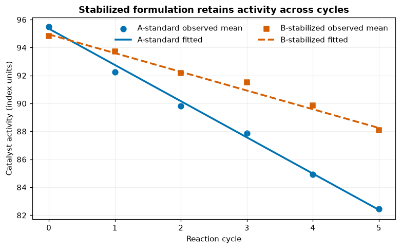
Stabilized formulation retains activity across cycles.

Interpretation. Both formulations deactivate, but the stabilized fitted line is less steep and ends higher. The close match between raw means and fitted lines is expected for this balanced synthetic design. The interaction, rather than the baseline formulation coefficient alone, answers the deactivation-rate question.

3.9. Step 5: inspect the fitted covariance

fitted_visit_covariance = np.asarray(mmrm_fit.extra["visit_covariance"])
fitted_rho = parameters["ar1_correlation"]
covariance_eigenvalues = np.linalg.eigvalsh(fitted_visit_covariance)
assert -1.0 < fitted_rho < 1.0
assert fitted_rho > 0.0
assert np.allclose(fitted_visit_covariance, fitted_visit_covariance.T)
assert np.all(covariance_eigenvalues > 0.0)

The fitted covariance is:

[[3.415 2.272 1.511 1.005 0.669 0.445]
 [2.272 3.415 2.272 1.511 1.005 0.669]
 [1.511 2.272 3.415 2.272 1.511 1.005]
 [1.005 1.511 2.272 3.415 2.272 1.511]
 [0.669 1.005 1.511 2.272 3.415 2.272]
 [0.445 0.669 1.005 1.511 2.272 3.415]]

Its eigenvalues are 0.7305, 0.8856, 1.2482, 2.1242, 4.5448, and 10.9587, all positive.

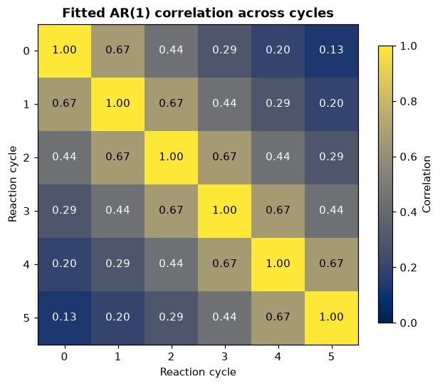
Fitted AR(1) correlation across cycles.

Interpretation. Correlation is one on the diagonal, strongest for adjacent cycles, and decays smoothly with lag. Positive definiteness establishes numerical validity of the fitted covariance; scientific suitability of AR(1) still depends on the experimental process.

3.10. Step 6: examine residuals by cycle

The committed cycle-specific residual summaries are:

Cycle	Mean residual	Residual SD
0	0.0056	1.7121
1	-0.1997	1.7046
2	-0.2124	1.8616
3	0.4487	2.1540
4	0.1057	1.9675
5	-0.0532	1.6524

print(f"{'cycle':>5s} {'mean residual':>15s} {'residual SD':>15s}")
for cycle_value in cycle_levels:
    selected = cycle == cycle_value
    cycle_residual = mmrm_fit.residuals[selected]
    print(
        f"{cycle_value:5.0f} "
        f"{float(np.mean(cycle_residual)):15.4f} "
        f"{float(np.std(cycle_residual, ddof=1)):15.4f}"
    )

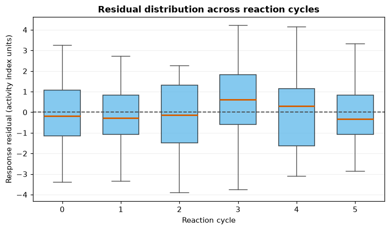
Residual distribution across reaction cycles.

Interpretation. Residual centers stay close to zero and spreads are broadly similar in this realization. This view supports, but does not replace, covariance sensitivity analysis and influence diagnostics.

3.11. Step 7: preserve covariance-axis provenance

The result manifest records REML, the model/data hashes, a deterministic-with-tolerance reproducibility class, the satterthwaite setting, and the resolved visit-order source. These fields make the covariance axis auditable independently of input row order.

3.12. API map

Task	Public API
Declare AR(1) covariance	pymixef.covariance.AR1
Declare the mean model	pymixef.model.Model.from_formula()
Preview compatibility	pymixef.model.Model.explain()
Compile and audit	pymixef.model.Model.compile(), pymixef.model.ExecutionPlan.explain()
Fit with REML	pymixef.model.ExecutionPlan.fit()
Read fixed and covariance estimates	pymixef.results.FitResult.parameters
Check convergence and Hessian diagnostics	pymixef.results.FitResult.convergence
Inspect visit order and covariance	pymixef.results.FitResult.extra
Read response residuals	pymixef.results.FitResult.residuals
Inspect provenance	pymixef.results.FitResult.manifest, pymixef.provenance.RunManifest.to_dict()

Interpretation boundaries

This example gives a transparent analysis of linear mean trajectories with homogeneous AR(1) residual covariance. For a discovery program, expand the same audited workflow with alternative mean curves and covariance structures, an explicit missingness rationale, preplanned contrasts, and physical diagnostics for poisoning, sintering, fouling, or phase change. The MMRM trajectory summarizes repeated activity; mechanistic experiments determine why that trajectory occurs and where it can be expected to transport.

3.13. Exercises

1. Replace AR(1) with pymixef.covariance.Unstructured and compare estimated covariance, parameter count, and convergence.

2. Try Toeplitz covariance and explain how lag-specific correlation differs from AR(1) decay.

3. Remove late-cycle measurements from selected catalysts. Audit exclusions and discuss whether missing at random is plausible.

4. Add I(cycle_centered ** 2) and inspect whether linear deactivation is adequate.

5. Permute the input rows and confirm that archived visit order and estimates remain invariant to numerical tolerance.

3.14. Takeaways

• Repeated-measures covariance encodes assumptions about within-unit dependence.

• Visit order must be explicit and auditable.

• The formulation-by-cycle interaction is the fitted slope difference.

• Check covariance positivity, convergence, and inference labels.

• Connect statistical trends back to mechanistic experiments.