6. Clustered binary response with a GLMM

Field: clinical and medical research
Analysis: Bernoulli-logit generalized linear mixed model (GLMM)
Clustering: patients nested within clinics
Reference engine: first-order Laplace approximation

Download the complete, pre-executed notebook

6.1. Domain and problem

Binary outcomes such as response/non-response, remission/no remission, or adverse-event/no adverse-event are common in multicenter studies. Patients treated at the same clinic may be more alike than patients treated at different clinics because of referral patterns, care pathways, or unmeasured site characteristics. A standard logistic regression does not represent that within-clinic dependence.

This tutorial uses a Bernoulli-logit GLMM with a clinic-level random intercept:

response ~ treatment + baseline_score + (1 | clinic)

The fixed effects estimate conditional treatment and baseline-score associations. The random intercept represents residual clinic-to-clinic heterogeneity on the log-odds scale.

For clinic \(j\) and patient \(i\), the fitted conditional probability is

\[ p_{ij} =\operatorname{logit}^{-1} \left(\beta_0+\beta_\mathrm{trt}\,\mathrm{trt}_{ij} +\beta_\mathrm{base}\,\mathrm{baseline}_{ij}+b_j\right), \qquad b_j\sim N(0,\sigma_b^2). \]

Consequently \(\exp(\beta_\mathrm{trt})\) is a clinic-conditional treatment odds ratio, not a marginal risk ratio.

6.2. What you will learn

By the end of the tutorial, you will be able to:

1. generate a deterministic clinic-clustered binary dataset;

2. select a Bernoulli likelihood and logit link through a public family object;

3. compile a model separately from fitting it;

4. inspect the design, model IR, data audit, and selected engine;

5. fit the supported Laplace reference GLMM and check trustworthy convergence;

6. translate fixed log-odds coefficients into conditional odds ratios;

7. review conditional response curves, in-sample calibration, and clinic conditional modes; and

8. ask PyMixEF to validate an unsupported AGHQ request without silently changing the requested method.

6.3. Dataset and model snapshot

Item	Value
Clinics	14
Patients per clinic	12
Analysis rows	168
Outcome	Binary response
Treatment allocation	84 control and 84 treatment observations
Additional predictor	Standardized continuous baseline score
Fixed effects	Intercept, treatment, baseline score
Random effects	Clinic-specific intercept
Family and link	Bernoulli with logit link
Engine and method	glmm, laplace
Seed	20260706

The synthetic generator uses an intercept of -0.55, a treatment log-odds effect of 0.80, a baseline-score effect of 0.45, and a clinic random-effect standard deviation of 0.55. Because outcomes are sampled, the fitted values need not reproduce those generating values exactly.

6.4. Runnable core analysis

The following excerpt is the core analysis from the executed notebook. It uses only ordinary Python and public PyMixEF APIs.

import numpy as np
from scipy.special import expit

import pymixef

SEED = 20260706
rng = np.random.default_rng(SEED)

n_clinics = 14
patients_per_clinic = 12
clinic_index = np.repeat(np.arange(n_clinics), patients_per_clinic)
n_rows = len(clinic_index)

treatment = np.tile(np.array([0, 1] * 6), n_clinics)
baseline_score = rng.normal(0.0, 1.0, n_rows)
clinic_intercept = rng.normal(0.0, 0.55, n_clinics)
linear_predictor = (
    -0.55
    + 0.80 * treatment
    + 0.45 * baseline_score
    + clinic_intercept[clinic_index]
)
generating_probability = expit(linear_predictor)
response = rng.binomial(1, generating_probability)

data = {
    "response": response,
    "treatment": treatment,
    "baseline_score": baseline_score,
    "clinic": np.array([f"C{i + 1:02d}" for i in clinic_index]),
}

model = pymixef.Model.from_formula(
    "response ~ treatment + baseline_score + (1 | clinic)",
    family=pymixef.families.Bernoulli(),
)
plan = model.compile(
    data,
    engine="glmm",
    method="laplace",
    maxiter=250,
    compute_hessian=False,
)
print(plan.explain())

fit = plan.fit()
assert fit.convergence.trustworthy, fit.convergence.to_dict()
print(fit.summary())

6.5. Step-by-step analysis

6.5.1. 1. Generate the clustered response

The generator balances treatment within every clinic, draws one latent log-odds shift per clinic, and then samples each response from its Bernoulli probability. The saved dataset has an overall observed response rate of 0.39880952380952384.

Balancing within clinic is useful here because the treatment contrast is not confounded with which clinics happened to enroll treated patients. Real data still require careful checks of allocation, missingness, and measured site-level differences.

6.5.2. 2. Compile before optimizing

Model.from_formula(...) records the statistical model. compile(...) binds it to the data, creates the fixed and random design matrices, validates engine compatibility, and produces an inspectable execution plan.

The saved plan reports:

• a fixed design of shape (168, 3) with rank 3;

• columns Intercept, treatment, and baseline_score;

• a clinic random design of shape (168, 1) across 14 groups;

• zero excluded source rows;

• a Bernoulli family with logit link;

• the requested glmm/laplace calculation path; and

• ModelIR hash c0306b40e2ee9601ce466dd518bf43684133ca7fe8b657721e4f7a8ae864e94e.

This separation lets an analysis review its design and calculation route before starting optimization.

6.5.3. 3. Fit and require trustworthy convergence

The notebook calls plan.fit() and asserts fit.convergence.trustworthy. The saved fit converged with objective 106.5094795 and log likelihood -106.5094795.

The recorded approximation is:

first-order Laplace at the joint conditional mode

The recorded quadrature order is 1; PyMixEF does not relabel that calculation as adaptive quadrature.

6.5.4. 4. Translate coefficients to conditional odds ratios

For a logit model, exponentiating a fixed coefficient produces an odds ratio conditional on the remaining predictors and on the clinic random intercept.

conditional_odds_ratios = {
    name: float(np.exp(value))
    for name, value in fit.parameters.items()
    if name in {"treatment", "baseline_score"}
}

assert conditional_odds_ratios["treatment"] > 1.0
print(conditional_odds_ratios)

The fitted treatment coefficient is 1.0520858, giving a conditional odds ratio of 2.863617891182583. The fitted baseline-score coefficient is 0.18998408, giving a conditional odds ratio of 1.2092303514690166 per one-unit increase in the standardized score.

6.5.5. 5. Inspect model-implied response curves

The fixed-effect predictor can be transformed through the inverse logit while setting the clinic random intercept to zero.

baseline_grid = np.linspace(-2.5, 2.5, 200)

for arm in (0, 1):
    curve_linear_predictor = (
        fit.parameters["Intercept"]
        + arm * fit.parameters["treatment"]
        + baseline_grid * fit.parameters["baseline_score"]
    )
    curve_probability = expit(curve_linear_predictor)

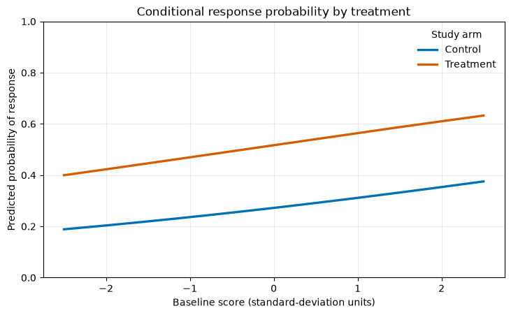
Conditional response probability by treatment. Fixed-effect predictions with the clinic random intercept set to zero.

Interpretation. Treatment shifts the conditional probability curve upward throughout the displayed baseline range. These are clinic-conditional curves at a random effect of zero, not population-marginal response probabilities.

6.5.6. 6. Compare observed and fitted rates

The archived fitted values are conditional fitted probabilities aligned to the analysis rows. Their arm-level averages are close to the observed rates:

Arm	N	Observed response rate	Mean fitted probability
Control (0)	84	0.2857142857142857	0.2798923202964317
Treatment (1)	84	0.5119047619047619	0.5140566349218681

Five fixed-width probability bins provide a compact descriptive calibration view.

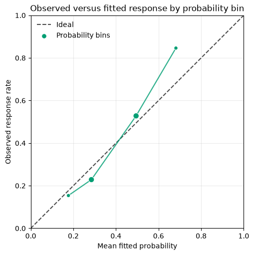
Observed versus fitted response by probability bin. Marker area reflects the number of patients in each nonempty bin.

Interpretation. The binned observations remain reasonably close to the diagonal for this synthetic dataset. This is an in-sample descriptive check; predictive calibration claims require held-out, cross-validated, or external data.

6.5.7. 7. Review clinic conditional modes

The random-effect diagnostic table exposes clinic names, conditional modes, and Laplace conditional standard deviations.

random_effect_diagnostics = fit.diagnostic("random_effects")
clinic_names = np.asarray(
    random_effect_diagnostics.columns["name"],
    dtype=str,
)
clinic_modes = np.asarray(
    random_effect_diagnostics.columns["conditional_mode"],
    dtype=float,
)
clinic_standard_deviations = np.asarray(
    random_effect_diagnostics.columns["conditional_sd_laplace"],
    dtype=float,
)

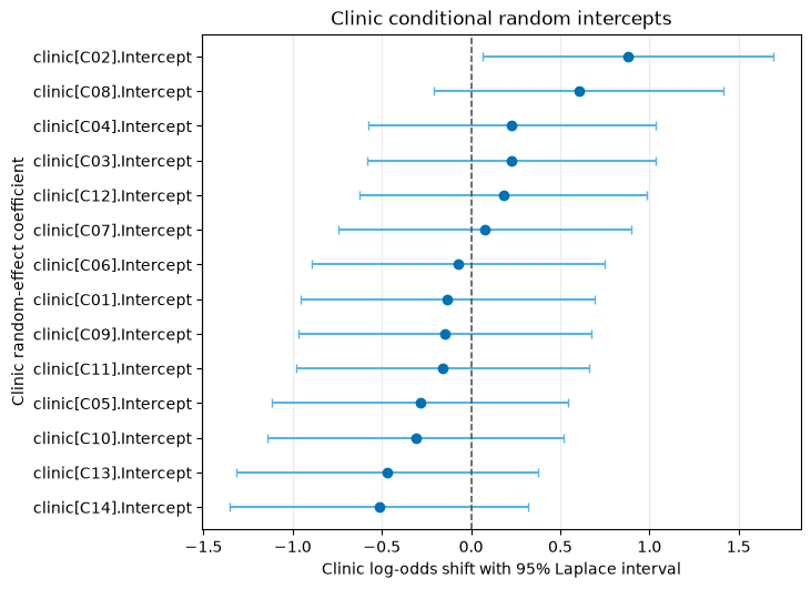
Clinic conditional random intercepts. Shrunken clinic log-odds shifts with 95% Laplace intervals.

Interpretation. The conditional modes vary around zero and their intervals overlap substantially, which is consistent with partial pooling. They summarize the fitted model’s clinic-specific shifts; they are not independently estimated clinic quality scores.

6.5.8. 8. Validate an unsupported calculation honestly

The model can be checked against an AGHQ request without performing optimization:

aghq_validation = model.validate(engine="aghq")
assert not aghq_validation.valid
assert any(
    item.code == "ENGINE-METHOD-002"
    for item in aghq_validation.findings
)

The saved finding is ENGINE-METHOD-002: the reference GLMM engine implements Laplace only, and AGHQ is not silently substituted.

6.6. Key saved results

Quantity	Saved value
Overall observed response rate	0.39880952380952384
Objective	106.5094795
Log likelihood	-106.5094795
Intercept	-0.98360725
Treatment coefficient	1.0520858
Baseline-score coefficient	0.18998408
Clinic random-intercept SD	0.5692520623280747
Conditional treatment odds ratio	2.863617891182583
Conditional baseline-score odds ratio	1.2092303514690166
Quadrature order recorded	1
Trustworthy convergence	True

6.7. API map

Task	Public API	Result used here
Declare a formula model	pymixef.model.Model.from_formula()	pymixef.model.Model
Select Bernoulli-logit behavior	pymixef.families.Bernoulli	pymixef.families.Family
Bind data and calculation controls	pymixef.model.Model.compile()	pymixef.model.ExecutionPlan
Inspect the compiled calculation	pymixef.model.ExecutionPlan.explain()	Human-readable plan
Fit the compiled model	pymixef.model.ExecutionPlan.fit()	pymixef.results.FitResult
Review convergence	pymixef.results.FitResult.convergence	pymixef.convergence.ConvergenceReport
Read coefficients	pymixef.results.FitResult.parameters	Named parameter mapping
Read row-aligned predictions	pymixef.results.FitResult.fitted_values	Conditional probabilities
Retrieve clinic modes	pymixef.results.FitResult.diagnostic()	pymixef.diagnostics.DiagnosticTable
Test engine compatibility	pymixef.model.Model.validate()	pymixef.model.ValidationReport

6.8. Exercises

1. Increase the generating clinic random-intercept standard deviation and compare it with the fitted variance component.

2. Reduce the number of patients per clinic and examine convergence and approximation stability.

3. Replace the binary outcomes with counts and use pymixef.families.Poisson().

4. Re-enable Hessian computation and review its diagnostics alongside optimizer termination.

5. Create a held-out clinic split and compare in-sample with out-of-clinic calibration.

Interpretation boundaries

Use this example as a transparent reference workflow for a small random-intercept Bernoulli GLMM. The displayed odds ratios are conditional effects, the calibration view is in-sample, and the clinic modes are pooled model summaries. The current dense first-order Laplace engine is experimental, and the notebook intentionally omits Hessian-based intervals. For a decision-bearing clinical analysis, add approximation-sensitivity work, pre-specified estimands, missing-data review, uncertainty intervals, and independent validation appropriate to the intended use.