5. Clinical-trial repeated measures with MMRM

This tutorial fits a Gaussian mixed model for repeated measures (MMRM) to deterministic synthetic change-from-baseline outcomes. It combines an arm-by-visit fixed-effects model, explicit within-subject AR(1) covariance, missing-response auditing, and visit-order provenance.

Download the executed notebook

5.1. What you will learn

The analysis shows how to:

• build a small randomized parallel-arm longitudinal dataset;

• represent within-subject covariance explicitly;

• audit outcomes omitted from the likelihood because they are missing;

• interpret reference-coded arm-by-visit coefficients;

• inspect estimated visit covariance and positive definiteness;

• derive an adjusted treatment contrast at each visit; and

• distinguish an educational reference fit from a confirmatory clinical analysis.

5.2. Domain question

Twenty-four subjects are assigned alternately to control or treated arms and measured at four ordered visits. The response is synthetic change from baseline. Four response values are set to missing to exercise the row-audit path.

The mean model is

\[ \text{change} \sim \text{baseline}+\text{treatment}\times\text{visit}. \]

The residual covariance is AR(1) within subject, so adjacent visits have the strongest residual association and correlation decays with visit separation.

5.3. Dataset snapshot

Property	Value
Subjects	24
Study arms	Control and treated
Ordered visits	0, 1, 2, 3
Planned rows	96
Observed outcomes	92
Missing outcomes	4
Generating residual SD	1.4
Generating AR-like correlation	0.55
Random seed	20260705

5.4. Reproduce the trial

The following excerpts are taken directly from the executed notebook and can be run from top to bottom.

import importlib
import logging

import numpy as np

import pymixef

# Keep a fresh-kernel run free of Matplotlib's one-time font-cache status message.
logging.getLogger("matplotlib.font_manager").setLevel(logging.ERROR)
plt = importlib.import_module("matplotlib.pyplot")

plt.style.use("tableau-colorblind10")

SEED = 20260705
rng = np.random.default_rng(SEED)

n_subjects = 24
visit_levels = np.arange(4, dtype=float)
subject_index = np.repeat(np.arange(n_subjects), len(visit_levels))
visit = np.tile(visit_levels, n_subjects)

arm_by_subject = np.array(
    ["control" if i % 2 == 0 else "treated" for i in range(n_subjects)]
)
treatment = np.repeat(arm_by_subject, len(visit_levels))
treated = np.repeat(
    (arm_by_subject == "treated").astype(float), len(visit_levels)
)
baseline_by_subject = rng.normal(18.0, 3.0, n_subjects)
baseline = np.repeat(baseline_by_subject, len(visit_levels))

generating_covariance = (
    1.4**2 * 0.55 ** np.abs(np.subtract.outer(visit_levels, visit_levels))
)
errors = np.concatenate(
    [
        rng.multivariate_normal(
            np.zeros(len(visit_levels)), generating_covariance
        )
        for _ in range(n_subjects)
    ]
)
change = (
    -0.15 * baseline
    + 0.25 * visit
    + 0.30 * treated
    + 0.35 * treated * visit
)
change = change + errors
change[[7, 18, 55, 86]] = np.nan

data = {
    "change": change,
    "baseline": baseline,
    "treatment": treatment,
    "visit": visit,
    "subject": np.array([f"S{i + 1:03d}" for i in subject_index]),
}

5.5. Step 1: inspect observed arm trajectories

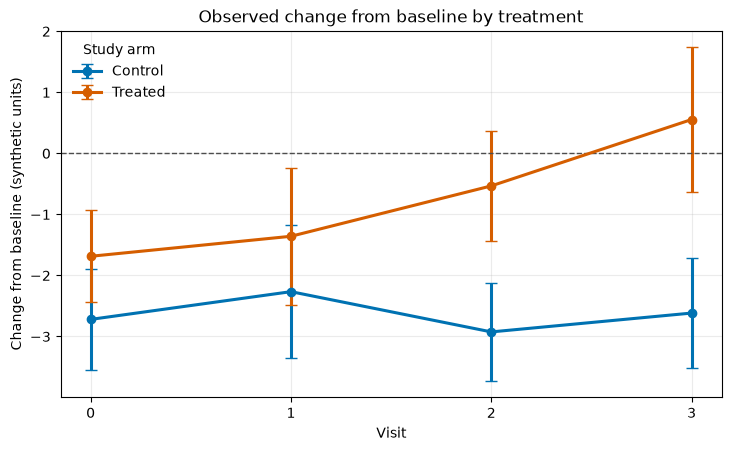
Observed change from baseline by treatment.

Interpretation. The treated arm separates progressively from control, matching the generated arm-by-visit effect. The error bars describe observed raw means and naturally reflect the four missing responses. MMRM adds baseline adjustment and a covariance model.

5.6. Step 2: declare covariance and compile

The covariance declaration identifies visit as the within-subject axis and subject as the grouping column. Numeric visit values resolve into ascending scientific order.

residual = pymixef.covariance.AR1(index="visit", group="subject")
model = pymixef.Model.from_formula(
    "change ~ baseline + treatment * visit",
    residual=residual,
)
plan = model.compile(
    data,
    engine="mmrm",
    method="reml",
    df_method="residual",
    maxiter=400,
    compute_hessian=False,
)
print(plan.explain())

The compiled audit reports:

Audit field	Saved value
Input rows	96
Analysis rows	92
Excluded rows	4
Retained-row reason	DATA-RETAINED-001: 92
Exclusion reason	DATA-MISSING-RESPONSE-001: 4
Fixed-design rank	5
Random formula blocks	None

The dedicated MMRM path places dependence in the residual covariance and does not combine this block with formula random effects.

5.7. Step 3: fit and verify visit-order provenance

fit = plan.fit()
assert fit.convergence.trustworthy, fit.convergence.to_dict()
print(fit.summary())
print("\nExcluded rows:", fit.extra["data_audit"]["excluded_rows"])
print("Visit levels:", fit.extra["visit_levels"])
print("Visit-order source:", fit.extra["visit_order_source"])

The result converges trustworthily. Visit levels are [0.0, 1.0, 2.0, 3.0], and the saved order source is ascending-explicit-visit-times.

The residual degrees-of-freedom setting is used because the optional Hessian is disabled. PyMixEF separately labels its available Satterthwaite and KR-inspired paths; a KR-inspired result is not silently described as exact Kenward–Roger.

5.7.1. Key saved results

Quantity	Estimate
Intercept	1.227748
Baseline coefficient	-0.214382
Treated-minus-control difference at visit 0	0.542230
Control-arm visit slope	0.011995
Treated-minus-control visit slope	0.712117
Residual SD	1.551934
AR(1) correlation	0.540353
Objective	160.4649943
Log likelihood	-160.4649943
Treated-minus-control difference at visit 3	2.678580655810124

The interaction controls how the adjusted treatment difference evolves:

\[ \widehat{\Delta}(v) =0.542230+0.712117v. \]

5.8. Step 4: inspect within-subject covariance

visit_covariance = np.asarray(fit.extra["visit_covariance"])
covariance_eigenvalues = np.linalg.eigvalsh(visit_covariance)
assert np.all(covariance_eigenvalues > 0), (
    "Visit covariance must be positive definite"
)
print("Estimated visit covariance:\n", np.round(visit_covariance, 3))
print("Eigenvalues:", np.round(covariance_eigenvalues, 6))

The saved covariance is:

[[2.408 1.301 0.703 0.380]
 [1.301 2.408 1.301 0.703]
 [0.703 1.301 2.408 1.301]
 [0.380 0.703 1.301 2.408]]

Its eigenvalues are 0.812723, 1.192278, 2.322836, and 5.306154. All are positive.

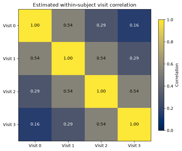
Estimated within-subject visit correlation.

Interpretation. Adjacent visits retain the strongest correlation and association decays with separation, as expected under AR(1). Explicit visit labels make covariance adjacency independent of input row order.

5.9. Step 5: calculate the final-visit contrast

Treatment coding is visible in parameter names. The main treatment term is the treated-minus-control difference at visit zero, and its interaction with visit is the additional treated slope.

treatment_term = next(
    name
    for name in fit.parameters
    if name.startswith("treatment[") and ":" not in name
)
interaction_term = next(
    name
    for name in fit.parameters
    if name.startswith("treatment[") and ":visit" in name
)
last_visit = float(max(fit.extra["visit_levels"]))
difference_at_last_visit = (
    fit.parameters[treatment_term]
    + last_visit * fit.parameters[interaction_term]
)
assert difference_at_last_visit > 0

The committed last-visit point estimate is 2.678580655810124 synthetic change units.

5.10. Step 6: construct contrasts with archived covariance

fixed_effect_names = list(fit.extra["fixed_effect_names"])
fixed_effect_covariance = np.asarray(fit.extra["fixed_effect_covariance"])
fixed_effect_vector = np.asarray(
    [fit.parameters[name] for name in fixed_effect_names]
)
contrast_estimates = []
contrast_standard_errors = []
for visit_level in visit_levels:
    contrast = np.zeros(len(fixed_effect_names))
    contrast[fixed_effect_names.index(treatment_term)] = 1.0
    contrast[fixed_effect_names.index(interaction_term)] = visit_level
    contrast_estimates.append(float(contrast @ fixed_effect_vector))
    contrast_standard_errors.append(
        float(np.sqrt(contrast @ fixed_effect_covariance @ contrast))
    )

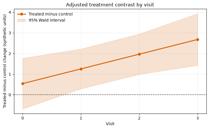
Adjusted treatment contrast by visit.

Interpretation. The adjusted treatment difference grows with visit, and the final-visit point estimate is positive. In a confirmatory analysis, both the target visit and interval method would be prespecified.

5.11. API map

Task	Public API
Declare within-subject AR(1)	pymixef.covariance.AR1
Declare the mean model	pymixef.model.Model.from_formula()
Compile, select DF handling, and audit	pymixef.model.Model.compile()
Explain the plan	pymixef.model.ExecutionPlan.explain()
Fit with REML	pymixef.model.ExecutionPlan.fit()
Check convergence	pymixef.results.FitResult.convergence
Read fixed and covariance parameters	pymixef.results.FitResult.parameters
Inspect missing-row audit	pymixef.results.FitResult.extra
Inspect visit axis and covariance	pymixef.results.FitResult.extra
Construct contrast uncertainty	pymixef.results.FitResult.extra

Interpretation boundaries

This example makes missing-response auditing, visit order, covariance, and longitudinal contrasts visible in one small analysis. A confirmatory workflow should add an explicitly defined estimand, a scientific missingness rationale, covariance sensitivity, prespecified target visits and multiplicity handling, the intended degrees-of-freedom procedure, and independent output validation. Model convergence confirms a numerical result; it does not by itself resolve missing-data bias or establish a clinical effect.

5.12. Exercises

1. Replace AR(1) with pymixef.covariance.Unstructured(index="visit", group="subject") and compare covariance estimates.

2. Increase missingness in one arm and discuss why model convergence does not resolve missing-data bias.

3. Use nonnumeric visit labels and provide an explicit scientific order before fitting an order-dependent covariance.

4. Re-enable the Hessian and use the explicitly labeled Satterthwaite option on this small dataset.

5.13. Takeaways

• Make the within-subject covariance and visit order explicit.

• Treat the missing-row audit as part of the analysis record.

• Interpret the treatment interaction as change in the arm contrast over visits.

• Check covariance positivity and convergence separately.

• Prespecify estimands and uncertainty procedures for confirmatory use.