10. Diagnostics, simulation, validation evidence, interchange, and archives

Field: longitudinal biomedical analysis and evidence engineering
Analysis: Gaussian random-intercept LMM with post-fit workflows
Lifecycle: diagnostics, simulation, archives, validation bundles, and interchange

Download the complete, pre-executed notebook

10.1. Domain and problem

Fitting a mixed-effects model is only one part of a reproducible analysis. Reviewers also need row-aligned diagnostics, seeded predictive simulations, portable results, integrity checks, traceability evidence, and explicit reports about what can and cannot be translated to another format.

This tutorial fits a small longitudinal LMM and then follows the fitted object through those supported post-fit workflows. The artifacts are created in a temporary directory and cleaned up at the end, so the example is safe to rerun.

10.2. What you will learn

By the end of the tutorial, you will be able to:

1. fit a reproducible random-intercept LMM;

2. retrieve machine-readable residual diagnostics;

3. generate new replicate datasets with a controlled seed;

4. create visual-predictive-check data;

5. save and verify a versioned non-pickle result archive;

6. create and verify a context-supporting validation evidence bundle;

7. use supported NONMEM-data, R-formula, and SED-ML interchange subsets; and

8. read integrity and compatibility reports conservatively.

10.3. Dataset and model snapshot

Item	Value
Subjects	10
Measurements per subject	4
Analysis rows	40
Time points	0, 1, 2, 3
Outcome	Continuous synthetic response
Fixed effects	Intercept and linear time
Random effects	Subject-specific intercept
Method	REML
Simulation seed	20260710
Predictive replicates	100
VPC bins	3

The fitted model is:

y ~ time + (1 | subject)

Equivalently, for observation \(j\) from subject \(i\),

\[ Y_{ij}=\beta_0+\beta_t t_{ij}+b_i+\epsilon_{ij}, \qquad b_i\sim N(0,\sigma_b^2), \qquad \epsilon_{ij}\sim N(0,\sigma^2). \]

A simulation replicate draws both latent and observation noise when those sources are enabled:

\[ Y_{ij}^{(r)} =\widehat\beta_0+\widehat\beta_t t_{ij} +b_i^{(r)}+\epsilon_{ij}^{(r)}. \]

10.4. Runnable core analysis

The following excerpt creates the data and fit used by every later section.

import numpy as np

import pymixef

SEED = 20260710
rng = np.random.default_rng(SEED)

subject_index = np.repeat(np.arange(10), 4)
time = np.tile(np.arange(4, dtype=float), 10)
random_intercept = rng.normal(0.0, 0.6, 10)
y = (
    2.0
    + 0.5 * time
    + random_intercept[subject_index]
    + rng.normal(0.0, 0.3, len(time))
)
data = {
    "y": y,
    "time": time,
    "subject": np.array(
        [f"S{i + 1:02d}" for i in subject_index]
    ),
}

fit = pymixef.fit(
    "y ~ time + (1 | subject)",
    data=data,
    method="reml",
    maxiter=300,
    compute_hessian=False,
)
print(fit.summary())

10.5. Step-by-step analysis

10.5.1. 1. Fit the reference LMM

The top-level pymixef.fit(...) helper parses the formula, compiles the model, and runs the requested reference engine. The saved fit converged with:

Quantity	Saved value
Objective	15.24635499
Log likelihood	-15.24635499
Intercept	1.3139967
Time coefficient	0.52977799
Subject random-intercept SD	0.37649945
Residual SD	0.24842785

The fitted object also retains calculation metadata used by the supported Gaussian simulation fallback.

10.5.2. 2. Retrieve row-aligned residual diagnostics

residuals = fit.residual_diagnostics()
raw = residuals.columns["raw_residual"]

print(residuals.name)
print(list(residuals.columns))
print(len(residuals))

The saved diagnostic is named residuals, contains 40 rows, and provides:

• row_id;

• observed;

• fitted;

• raw_residual; and

• pearson_residual.

The saved raw-residual mean is -2.7755575615628915e-18, numerically zero, and the raw-residual RMSE is 0.2147265492857147.

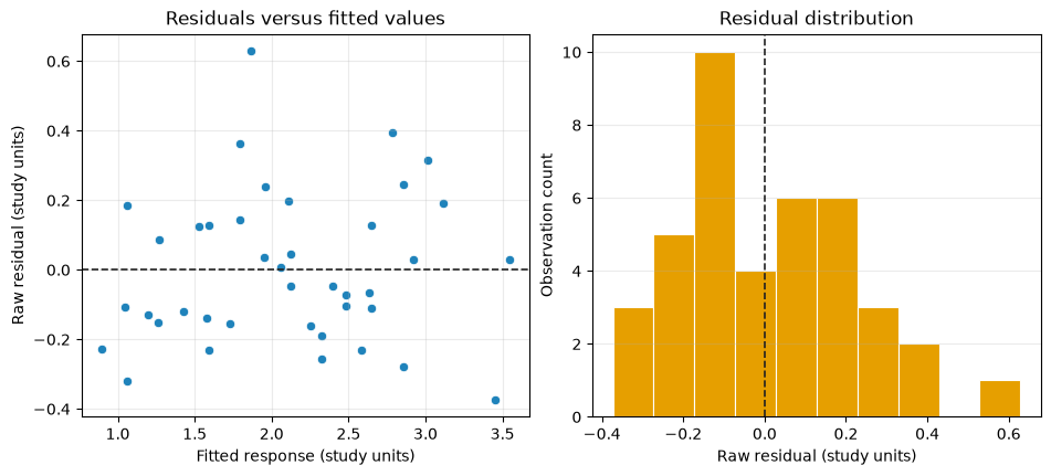
Residuals versus fitted values and residual distribution. A zero reference line anchors both the scatterplot and histogram.

Interpretation. Residuals are centered near zero without a strong visible fitted-value trend in this small synthetic example. The views guide structured review; they do not by themselves prove normality, constant variance, or external model adequacy.

10.5.3. 3. Generate seeded new-replicate simulations

FitResult.simulate(...) draws new Gaussian longitudinal datasets from the full archived observation covariance. It does not repeat the fitted-value vector.

simulations = fit.simulate(
    n_replicates=100,
    seed=SEED,
)
repeat_simulations = fit.simulate(
    n_replicates=100,
    seed=SEED,
)

assert np.array_equal(simulations, repeat_simulations)
assert simulations.shape == (100, 40)

The same seed produces byte-for-byte identical arrays in this execution. A different seed should produce a different set of replicate datasets.

10.5.4. 4. Build and visualize VPC data

vpc = fit.vpc(
    bins=3,
    simulations=100,
    seed=SEED,
)

print(list(vpc.columns))
print(len(vpc))

The helper returns nine rows: three quantiles (0.05, 0.50, and 0.95) for each of three ordered-index bins. Its columns are:

bin, bin_left, bin_right, quantile, observed, simulated_median,
simulated_lower, simulated_upper, n_observed

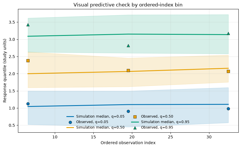
Visual predictive check by ordered-index bin. Observed quantile markers are overlaid on seeded simulation medians and interval bands.

Interpretation. The observed 5th, 50th, and 95th percentile markers remain inside the simulated envelopes in this execution. This is a useful visual calibration check, not a formal acceptance threshold.

The notebook also summarizes each replicate by its sample mean:

simulated_means = np.mean(simulations, axis=1)
observed_mean = float(np.mean(y))
mean_interval = np.quantile(
    simulated_means,
    [0.05, 0.95],
)

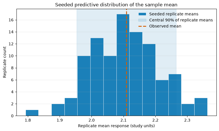
Seeded predictive distribution of the sample mean. The observed mean is compared with the central 90% of new-replicate means.

Interpretation. Replicate means vary because every simulation draws a new longitudinal dataset using the archived covariance. This is one predictive summary and complements rather than replaces subject-level and residual diagnostics.

10.5.5. 5. Save and verify a versioned result archive

PyMixEF saves JSON rather than pickle and writes a whole-file SHA-256 sidecar.

from pathlib import Path
from tempfile import TemporaryDirectory

temporary_workspace = TemporaryDirectory()
artifact_dir = Path(temporary_workspace.name)

result_path = fit.save(artifact_dir / "fit.json")
reloaded = pymixef.FitResult.load(
    result_path,
    require_sidecar=True,
)

assert result_path.exists()
assert result_path.with_suffix(".json.sha256").exists()
assert reloaded.parameters == fit.parameters

With require_sidecar=True, loading checks the sidecar, manifest output hashes, and the manifest’s semantic ModelIR hash. The saved ModelIR hash is:

sha256:994469709cdb83a52fc456801afd8805dd7c48f4af9d5cc64833c5ab26f4aad5

10.5.6. 6. Create a validation evidence bundle

bundle_path = pymixef.create_validation_bundle(
    fit,
    artifact_dir / "validation-bundle.zip",
    analysis_data=data,
    include_data=False,
)
bundle_check = pymixef.verify_validation_bundle(
    bundle_path
)
assert bundle_check["valid"]

The verified bundle contains:

• README.txt;

• manifest.json;

• result.json; and

• traceability.json.

Its recorded engine is lmm. The saved analysis-data hash is:

sha256:3a33c9ef1ebf788ea3cd4ac68c5941dfb0642be511f5392b345a91c17a1bedb3

Raw analysis data are excluded because include_data=False; the hash provides a link to the analyzed content without placing those records into the archive.

10.5.7. 7. Use conservative interchange subsets

Each interchange operation returns a value and a compatibility report.

from pymixef.interoperability import (
    export_sedml,
    import_nonmem_data,
    import_sedml,
    translate_r_formula,
)

nonmem_data = import_nonmem_data(
    {
        "id": [1, 1],
        "time": [0, 1],
        "dv": [2.0, 1.5],
    }
)
formula_translation = translate_r_formula(
    "y ~ time + (1 | subject)"
)

sedml_path = artifact_dir / "design.xml"
sedml_export = export_sedml(
    {
        "output_end_time": 24.0,
        "number_of_points": 24,
    },
    sedml_path,
)
sedml_design = import_sedml(
    sedml_path
).require_supported()

assert nonmem_data.report.supported
assert formula_translation.report.supported
assert sedml_export.report.supported

The saved SED-ML simulation is:

{
    "id": "simulation",
    "initial_time": 0.0,
    "output_start_time": 0.0,
    "output_end_time": 24.0,
    "number_of_points": 24,
    "algorithm": "KISAO:0000019",
}

The standard NONMEM-style names, ordinary mixed-model formula, and uniform time-course SED-ML design are all reported as supported.

10.5.8. 8. Review explicit refusals

PyMixEF does not execute arbitrary R code or guess at the columns generated by R functions:

unsupported_formula = translate_r_formula(
    "y ~ poly(time, 2) + (1 | subject)"
)
assert not unsupported_formula.report.supported

unsupported_issues = [
    issue.to_dict()
    for issue in unsupported_formula.report.by_status(
        "unsupported"
    )
]

The saved issue identifies poly( and instructs the analyst to create the transformed column explicitly.

The notebook finally calls temporary_workspace.cleanup() so no temporary artifact survives the example.

10.6. Key saved results

Workflow	Saved result
LMM convergence	Converged
Simulation shape	(100, 40)
Same-seed identity	True
VPC rows	9
Result JSON exists	True
SHA-256 sidecar exists	True
Reloaded parameters preserved	True
Validation bundle valid	True
Bundle engine	lmm
NONMEM-data support	True
R-formula support	True
SED-ML export support	True
R poly(...) support	False

10.7. API map

Task	Public API	Result used here
Fit a formula model	pymixef.model.fit()	pymixef.results.FitResult
Render fit summary	pymixef.results.FitResult.summary()	Text summary
Retrieve residuals	pymixef.results.FitResult.residual_diagnostics()	pymixef.diagnostics.DiagnosticTable
Generate new replicates	pymixef.results.FitResult.simulate()	Replicate-by-row array
Build VPC data	pymixef.results.FitResult.vpc()	Quantile pymixef.diagnostics.DiagnosticTable
Save result	pymixef.results.FitResult.save()	JSON path plus sidecar
Verify/reload result	pymixef.results.FitResult.load()	Reconstructed result
Create evidence bundle	pymixef.validation.create_validation_bundle()	ZIP archive
Verify evidence bundle	pymixef.validation.verify_validation_bundle()	Verification mapping
Import NONMEM-style data	pymixef.interoperability.nonmem.import_nonmem_data()	pymixef.interoperability.base.InterchangeResult
Translate R formula subset	pymixef.interoperability.r.translate_r_formula()	pymixef.interoperability.base.InterchangeResult
Export SED-ML subset	pymixef.interoperability.sedml.export_sedml()	pymixef.interoperability.base.InterchangeResult
Import SED-ML subset	pymixef.interoperability.sedml.import_sedml()	pymixef.interoperability.base.InterchangeResult
Require supported result	pymixef.interoperability.base.InterchangeResult.require_supported()	Translated value
Filter compatibility issues	pymixef.interoperability.base.CompatibilityReport.by_status()	Issue tuple

10.8. Exercises

1. Change the simulation seed and compare reproducibility within and across seeds.

2. Save a result, alter a copy of its JSON, and confirm that loading the altered copy fails integrity verification.

3. Include synthetic analysis data in a validation bundle and inspect its member list. Do not include sensitive data without authorization.

4. Add an unsupported construct to an interchange example and report the explicit refusal.

5. Increase the number of VPC simulations and compare interval stability while retaining the seed and bin definition in the analysis record.

Interpretation boundaries

Use these tools to strengthen an evidence workflow: diagnostics guide review, seeded simulation supports reproducible predictive checks, hashes detect inconsistent artifacts, bundles preserve context, and compatibility reports make translation decisions visible. Hashes are integrity checks rather than digital signatures, and a validation bundle contributes evidence rather than serving as a universal regulatory certificate. Review the report before calling require_supported(), protect any included analysis data, and add context-specific validation for the intended use.