9. Pharmacometric declarations and the shared ModelIR

Field: population pharmacokinetics and model engineering
Analysis: typed model declaration and semantic compilation
Model: one-compartment PK with weight on clearance
Output: versioned, backend-neutral ModelIR

Download the complete, pre-executed notebook

9.1. Domain and problem

A pharmacometric model needs more than equations. Parameters require domains and optimizer transforms, random effects need covariance and level semantics, states need units and initial values, doses need event mappings, and observations need likelihoods. If those meanings exist only in handwritten code, it is difficult to compare, serialize, audit, or route the model to a compatible backend.

This tutorial declares a one-compartment population-PK model with PyMixEF’s typed Python DSL. It validates the declaration, translates it to the same versioned pymixef.ir.ModelIR used by formula models, visualizes structural dependencies, and proves deterministic semantic identity after a JSON round-trip.

The central structural equations are

\[ CL_i=TVCL\left(\frac{WT_i}{70}\right)^{0.75}\exp(\eta_{CL,i}), \qquad \eta_{CL,i}\sim N(0,\omega_{CL}^2), \]

\[ \frac{dA_i(t)}{dt}=-\frac{CL_i}{V}A_i(t), \qquad f_i(t)=\frac{A_i(t)}{V}, \qquad Y_i(t)\mid f_i(t)\sim N\!\left(f_i(t),\sigma^2\right). \]

The declaration records these meanings as typed graph nodes instead of leaving them implicit in executable Python.

9.2. What you will learn

By the end of the tutorial, you will be able to:

1. declare positive parameters with initial values and units;

2. declare a subject-level random effect and a referenced covariate;

3. build an allometric clearance expression;

4. declare a state, dose mapping, differential equation, and observation model;

5. inspect and validate a compiled declaration without fitting it;

6. read estimator compatibility without substituting unavailable estimators;

7. translate the declaration into explicit ModelIR node families;

8. inspect direct and propagated structural dependencies; and

9. serialize, reload, compare, and hash the complete model meaning.

9.3. Model snapshot

Component	Declaration
Typical clearance	tvcl=5.0 L/h, positive
Volume	volume=25.0 L, positive
Additive residual SD	sigma=0.2 mg/L, positive
Random effect	eta_cl, subject level, diagonal block omega_cl
Covariate	Weight in kg, reference 70 kg
Clearance relationship	tvcl * (weight / 70) ** 0.75 * exp(eta_cl)
State	Central amount in mg, initial value 0
State equation	First-order elimination
Dose mapping	AMT/RATE/DUR into central, IV route
Observation	DV, mean central / volume, additive error
DSL schema	1.0
ModelIR schema	1.0.0

The weight exponent of 0.75 is an illustrative allometric relationship, not a universal covariate model.

9.4. Runnable core declaration

This is the exact typed declaration from the executed notebook:

from pymixef.pharmacometrics import (
    Dose,
    Eta,
    Param,
    State,
    additive,
    covariate,
    d,
    exp,
    observe,
)
from pymixef.pharmacometrics import model as pm_model


@pm_model
def population_pk():
    tvcl = Param.positive("tvcl", init=5.0, unit="L/h")
    volume = Param.positive("volume", init=25.0, unit="L")
    sigma = Param.positive("sigma", init=0.2, unit="mg/L")
    (eta_cl,) = Eta.independent("eta_cl", block="omega_cl")

    weight = covariate("weight", unit="kg", reference=70.0)
    clearance = tvcl * (weight / 70.0) ** 0.75 * exp(eta_cl)

    central = State("central", unit="mg")
    Dose.into(central, amount="AMT", rate="RATE")
    d(central, -(clearance / volume) * central)
    observe("DV", mean=central / volume, error=additive(sigma))


compiled = population_pk()
print(compiled.explain())

validation = compiled.validate()
assert validation.valid

model_ir = compiled.to_ir()

The decorator executes the Python declarations to build a data-only expression tree. Calling population_pk() compiles that declaration; it does not estimate population parameters.

9.5. Step-by-step analysis

9.5.1. 1. Declare constrained parameters

Param.positive(...) gives each parameter:

• positive support;

• a log optimizer transform;

• an initial value;

• an optional scientific unit; and

• the population-parameter role.

For example, the saved tvcl node contains:

{
    "node_type": "parameter",
    "support": "positive",
    "transform": "log",
    "unit": "L/h",
    "name": "tvcl",
    "initial": 5.0,
    "bounds": [0.0, None],
    "fixed": False,
    "role": "population-parameter",
}

9.5.2. 2. Connect the covariate and random effect

Eta.independent(...) creates one subject-level Gaussian random effect in a diagonal covariance block. covariate(...) records weight, its unit, and its 70 kg reference. The expression system retains the full clearance dependency:

tvcl * (weight / 70.0) ** 0.75 * exp(eta_cl)

9.5.3. 3. Declare state dynamics, dose semantics, and observation

The central state uses amount units. Dose.into(...) maps standard dose fields into that state. d(...) records the ODE, and observe(...) maps the state to the DV response through concentration and additive error.

The compiled explanation reports:

d(central)/dt =
    -((tvcl * (weight / 70.0) ** 0.75 * exp(eta_cl)) / volume)
    * central

The serialized state-equation node has direct dependencies on central, eta_cl, tvcl, volume, and weight.

9.5.4. 4. Validate capability before choosing an estimator

validation = compiled.validate()
assert validation.valid, [
    message.to_dict()
    for message in validation.messages
]

print(dict(validation.estimator_compatibility))

The saved compatibility map is:

Capability	Available
Simulation	True
Conditional mode	True
Production FOCEI fit	False
SAEM	False

There are no validation messages for the declaration itself. Compatibility is reported separately so syntactic validity is not mistaken for availability of every estimation algorithm.

9.5.5. 5. Translate to the shared ModelIR

compiled.to_ir() emits explicit typed nodes. The saved node summary is:

IR collection	Saved contents
Source	pharmacometrics-dsl
Parameters	tvcl, volume, sigma
Random-effect groups	subject
Predictors	weight
State equations	central
Event types	dose-mapping
Likelihood responses	DV
Outputs	DV_prediction

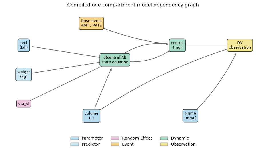
Compiled one-compartment model dependency graph. Colors distinguish parameters, predictors, random effects, events, dynamics, and observations.

Interpretation. Dose fields update the central state; clearance determinants feed its differential equation; and central amount, volume, and residual scale feed the observation. The two arrows between the ODE and central state depict numerical integration of a state-dependent equation, not another statistical effect.

9.5.6. 6. Inventory the explicit semantic components

The executed notebook counts the node families rather than treating the model as an opaque function.

ModelIR component	Count
Parameters	3
Random-effect groups	1
Predictors	1
State equations	1
Event mappings	1
Likelihoods	1
Transforms	3
Outputs	1

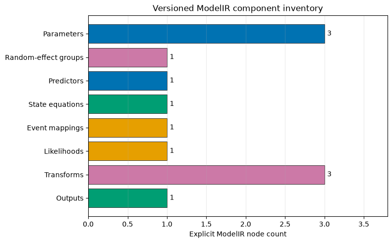
Versioned ModelIR component inventory. Every declared scientific or optimizer concept remains an explicit node.

Interpretation. Each positive parameter receives an explicit optimizer transform. Dynamics, event mapping, likelihood, and output remain individually visible. The counts describe representation structure; they do not by themselves establish identifiability or estimation readiness.

9.5.7. 7. Distinguish direct from propagated dependencies

The incidence matrix uses each IR node’s dependencies collection.

state_equation = model_ir.state_equations[0]
event_mapping = model_ir.events[0]
likelihood_node = model_ir.likelihoods[0]
output_node = model_ir.outputs[0]

dependency_symbols = (
    [node.name for node in model_ir.parameters]
    + [
        term
        for group in model_ir.random_effects
        for term in group.terms
    ]
    + [node.name for node in model_ir.predictors]
    + [state_equation.state]
)

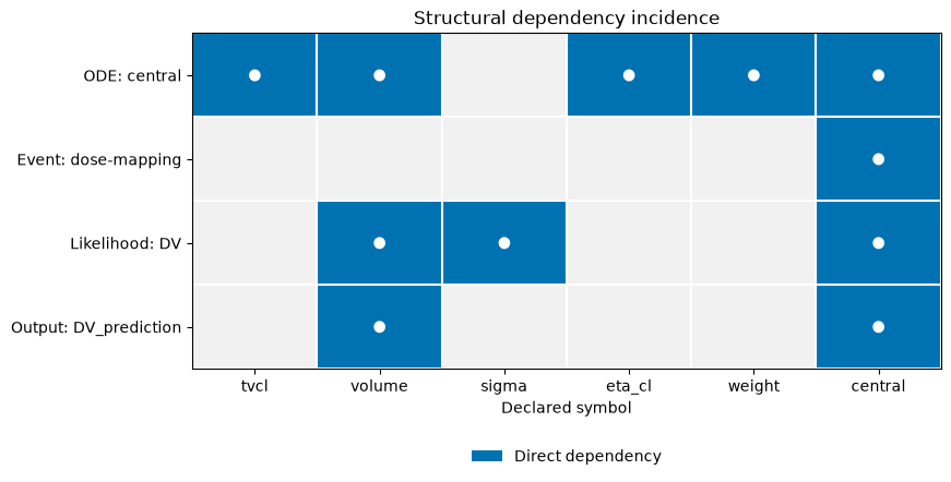
Structural dependency incidence. Filled cells denote direct dependencies recorded by each typed IR node.

Interpretation. tvcl, weight, and eta_cl directly affect the ODE. The likelihood depends on them only through the central state, while sigma enters the likelihood directly. This separates direct edges from relationships propagated through intermediate nodes.

9.5.8. 8. Perform a semantic JSON round-trip

Canonical serialization carries the full versioned IR meaning.

from pymixef import ModelIR

serialized = model_ir.to_json(indent=2)
reloaded = ModelIR.from_json(serialized)

assert reloaded == model_ir
assert reloaded.semantic_hash == model_ir.semantic_hash

The saved round-trip result is:

• semantic hash: 41c72acbf7b36c34accdb741f0470fef03e290e58bd8ce74523d6d6d4edf01a7;

• equality after reload: True;

• semantic hash preserved: True; and

• indented JSON length: 10367 characters.

Equality compares semantic model content, not Python object identity.

9.6. Key saved results

Quantity	Saved value
Declaration validation	True
Simulation compatibility	True
Conditional-mode compatibility	True
Production FOCEI compatibility	False
SAEM compatibility	False
ModelIR schema	1.0.0
ModelIR source	pharmacometrics-dsl
Parameter count	3
Transform count	3
Semantic hash	41c72acbf7b36c34accdb741f0470fef03e290e58bd8ce74523d6d6d4edf01a7
Round-trip equality	True
JSON length	10367 characters

9.7. API map

Task	Public API	Result used here
Define a model	pymixef.pharmacometrics.dsl.model()	Model decorator
Declare positive parameter	pymixef.pharmacometrics.dsl.Param.positive()	Typed parameter expression
Declare independent ETA	pymixef.pharmacometrics.dsl.Eta.independent()	Random-effect expression
Declare a covariate	pymixef.pharmacometrics.dsl.covariate()	Predictor expression
Apply exponential transform	pymixef.pharmacometrics.dsl.exp()	Expression node
Declare state	pymixef.pharmacometrics.dsl.State	State expression
Map dose fields	pymixef.pharmacometrics.dsl.Dose.into()	Event mapping
Declare state derivative	pymixef.pharmacometrics.dsl.d()	Differential equation
Declare observation	pymixef.pharmacometrics.dsl.observe()	Observation mapping
Declare additive error	pymixef.pharmacometrics.pk.additive()	Observation-error expression
Inspect declaration	pymixef.pharmacometrics.dsl.CompiledModel.explain()	Text explanation
Validate declaration	pymixef.pharmacometrics.dsl.CompiledModel.validate()	pymixef.pharmacometrics.dsl.ModelValidation
Compile semantic IR	pymixef.pharmacometrics.dsl.CompiledModel.to_ir()	pymixef.ir.ModelIR
Serialize model	pymixef.ir.ModelIR.to_json()	Canonical JSON
Reload model	pymixef.ir.ModelIR.from_json()	Reconstructed pymixef.ir.ModelIR
Compare semantic identity	pymixef.ir.ModelIR.semantic_hash	SHA-256-style identity
Inspect individual nodes	pymixef.ir.IRNode.to_dict()	Plain Python mapping

9.8. Exercises

1. Add a proportional component to the observation error and inspect the resulting likelihood node.

2. Add a random effect on volume and compare independent with correlated block declarations.

3. Change the weight exponent and confirm that the semantic hash changes.

4. Serialize the IR twice and verify that the canonical JSON strings are identical.

5. Change only a parameter’s initial value, then use the IR representations to identify exactly what changed.

Interpretation boundaries

Use the DSL and ModelIR as an auditable model contract: they make declarations, dependencies, transforms, and event/observation semantics explicit. A valid contract is an essential prerequisite, but it is not a fitted population analysis or evidence of parameter identifiability. The current compatibility report intentionally keeps production FOCEI and SAEM unavailable, does not perform automatic unit conversion, and refuses opaque constructs. Estimation qualification, data diagnostics, and external evidence should be added for the intended scientific or regulated use.