2. Binary catalyst success with a generalized mixed model

Some catalyst-screening endpoints are binary: an activation run reaches a conversion threshold, or it does not. Repeated runs from the same catalyst lot are correlated, so an ordinary logistic regression can understate lot-to-lot clustering. This tutorial fits a Bernoulli generalized linear mixed model (GLMM) with a random lot intercept.

Download the executed notebook

2.1. What you will learn

This analysis shows how to:

• generate deterministic clustered binary data;

• connect log-odds coefficients, conditional odds ratios, and probabilities;

• fit PyMixEF’s Bernoulli-logit first-order Laplace path;

• inspect outer-optimizer and conditional-mode convergence;

• distinguish typical-lot conditional predictions from marginalized population probabilities;

• inspect shrunken lot modes; and

• tell an in-sample calibration diagnostic apart from out-of-lot validation.

2.2. Domain question

Twelve catalyst lots each undergo eight activation runs. Every lot is tested with and without a promoter, and standardized temperature varies by run. The conditional model is

\[ \operatorname{logit}\{P(Y_{ij}=1\mid b_j)\} =\beta_0+\beta_T T_{ij}+\beta_P P_{ij}+b_j. \]

The random intercept \(b_j\) represents persistent lot-level shifts in activation propensity after accounting for temperature and promoter use.

2.3. Dataset snapshot

Property	Value
Analysis rows	96
Catalyst lots	12
Runs per lot	8
Outcome	Binary success
Promoter-off successes	20/48 (0.417)
Promoter-on successes	31/48 (0.646)
Overall success rate	0.531
Generating lot-intercept SD	0.45
Random seed	30

2.4. Reproduce the data

Run the excerpts in order. They are taken directly from the executed notebook.

import importlib
import logging
from pprint import pprint

import numpy as np

import pymixef

# Keep first-run Matplotlib font-cache status out of committed showcase output.
logging.getLogger("matplotlib.font_manager").setLevel(logging.ERROR)
plt = importlib.import_module("matplotlib.pyplot")

print("PyMixEF version:", pymixef.__version__)

plt.rcParams.update(
    {
        "figure.dpi": 110,
        "font.size": 10,
        "axes.titleweight": "semibold",
    }
)

rng = np.random.default_rng(30)

n_lots = 12
runs_per_lot = 8
lot_index = np.repeat(np.arange(n_lots), runs_per_lot)
catalyst_lot = np.array([f"lot-{index + 1:02d}" for index in lot_index])
temperature_scaled = rng.normal(size=lot_index.size)
promoter = np.tile([0, 1, 0, 1, 0, 1, 0, 1], n_lots)

lot_intercept = rng.normal(0.0, 0.45, n_lots)
linear_predictor = (
    -0.30
    + 0.55 * temperature_scaled
    + 0.45 * promoter
    + lot_intercept[lot_index]
)
success_probability = 1.0 / (1.0 + np.exp(-linear_predictor))
success = rng.binomial(1, success_probability)

binary_data = {
    "success": success,
    "temperature_scaled": temperature_scaled,
    "promoter": promoter,
    "catalyst_lot": catalyst_lot,
}

The generated probabilities are not passed to the model; they are retained only because this is a simulation. The fitted analysis receives the binary outcome and observed predictors.

2.5. Step 1: declare the Bernoulli-logit model

pymixef.families.Bernoulli() selects the canonical logit link. The (1 | catalyst_lot) term creates the lot-level random intercept.

glmm_model = pymixef.Model.from_formula(
    "success ~ temperature_scaled + promoter + (1 | catalyst_lot)",
    family=pymixef.families.Bernoulli(),
)

print(
    glmm_model.explain(
        binary_data,
        engine="glmm",
        method="laplace",
    )
)

The explanation reports a rank-three fixed design, 12 lot groups, 96 retained rows, a Bernoulli family with logit link, and valid GLMM/Laplace compatibility.

2.6. Step 2: compile and audit

glmm_plan = glmm_model.compile(
    binary_data,
    engine="glmm",
    method="laplace",
    maxiter=400,
)

print(glmm_plan.explain())
pprint(
    {
        "analysis_rows": glmm_plan.matrices.audit.analysis_rows,
        "excluded_rows": glmm_plan.matrices.audit.excluded_rows,
        "fixed_columns": glmm_plan.matrices.fixed_names,
        "random_blocks": len(glmm_plan.matrices.random_blocks),
    }
)

The audit retains every row. Fixed columns are Intercept, temperature_scaled, and promoter; there is one random-effect block.

2.7. Step 3: fit the first-order Laplace approximation

Laplace integration approximates the random-effect integral by expanding near the joint conditional mode.

glmm_fit = glmm_plan.fit()
print(glmm_fit.summary())

convergence = glmm_fit.convergence
pprint(
    {
        "status": convergence.status,
        "trustworthy": convergence.trustworthy,
        "optimizer_terminated": convergence.optimizer_terminated,
        "scaled_gradient_inf_norm": convergence.scaled_gradient_inf_norm,
        "conditional_mode_failures": convergence.conditional_mode_failures,
        "warning_codes": [warning.code for warning in convergence.warnings],
        "approximation": glmm_fit.extra["approximation"],
        "quadrature_order": glmm_fit.extra["quadrature_order"],
    }
)

assert convergence.trustworthy, "Review convergence before interpretation."
assert convergence.conditional_mode_failures == 0

The committed fit is trustworthy, has no warning codes or conditional-mode failures, and records a scaled-gradient infinity norm of 3.126388037363008e-05. Its approximation is first-order Laplace at the joint conditional mode, with quadrature order one.

2.8. Step 4: interpret log-odds and odds ratios

Exponentiating a coefficient gives a conditional odds ratio with the lot random effect and other predictors held constant.

fixed_effect_names = ["Intercept", "temperature_scaled", "promoter"]
print(f"{'term':24s} {'log-odds':>12s} {'odds ratio':>12s}")
for name in fixed_effect_names:
    estimate = glmm_fit.parameters[name]
    print(f"{name:24s} {estimate:12.4f} {np.exp(estimate):12.4f}")

promoter_odds_ratio = np.exp(glmm_fit.parameters["promoter"])
assert promoter_odds_ratio > 1.0, "The synthetic promoter effect should raise the odds."

2.8.1. Key saved results

Quantity	Estimate
Intercept log-odds	-0.4571
Intercept odds	0.6331
Temperature log-odds coefficient	0.4513
Temperature conditional odds ratio	1.5703
Promoter log-odds coefficient	1.2061
Promoter conditional odds ratio	3.3405
Lot random-intercept SD	0.9927
Objective	59.81036004
Log likelihood	-59.81036004

An odds ratio of 3.3405 is not a probability ratio. The probability difference depends on the starting log odds and therefore on temperature and lot effect.

2.9. Step 5: translate the fixed effects to typical-lot probabilities

Setting the lot random intercept to zero yields a conditional illustration for a typical lot.

def logistic(value):
    return 1.0 / (1.0 + np.exp(-value))


beta0 = glmm_fit.parameters["Intercept"]
beta_temperature = glmm_fit.parameters["temperature_scaled"]
beta_promoter = glmm_fit.parameters["promoter"]

print(f"{'temperature z':>13s} {'promoter':>10s} {'probability':>13s}")
for temperature_value in (-1.0, 0.0, 1.0):
    for promoter_value in (0, 1):
        eta = (
            beta0
            + beta_temperature * temperature_value
            + beta_promoter * promoter_value
        )
        print(
            f"{temperature_value:13.1f} "
            f"{promoter_value:10d} "
            f"{logistic(eta):13.3f}"
        )

Standardized temperature	No promoter	Promoter
-1	0.287	0.574
0	0.388	0.679
1	0.499	0.769

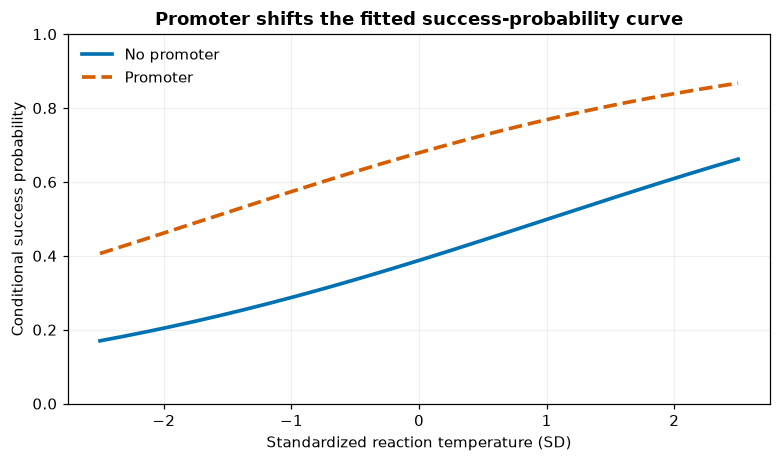
Promoter shifts the fitted success-probability curve.

Interpretation. Across the displayed temperature range, promoter use moves the fitted conditional probability upward for a lot whose random intercept is zero. These curves are not fully marginalized population probabilities, because integration over a random effect and the nonlinear logistic transformation do not commute.

2.10. Step 6: inspect lot modes

sorted_lot_modes = sorted(
    glmm_fit.random_effects.items(),
    key=lambda item: item[1],
)
assert all(np.isfinite(mode) for _, mode in sorted_lot_modes)
print("Three lowest conditional lot modes:")
pprint(sorted_lot_modes[:3])
print("Three highest conditional lot modes:")
pprint(sorted_lot_modes[-3:])

The lowest saved modes are lot-02 at -1.3050, lot-03 at -0.8458, and lot-01 at -0.5978. The highest are lot-08 at 0.7618, lot-10 at 0.9358, and lot-11 at 1.4328.

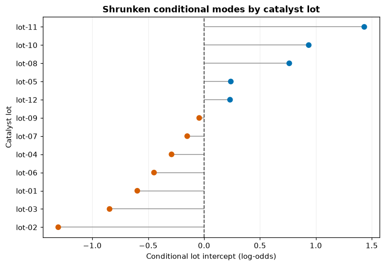
Shrunken conditional modes by catalyst lot.

Interpretation. The lots vary around the population intercept, and mixed model shrinkage pulls the estimates toward zero. Conditional modes are model-based estimates, not observed or permanent quality scores for future lots.

2.11. Step 7: assess in-sample conditional calibration

fitted_probability = np.asarray(glmm_fit.fitted_values)
assert np.all((fitted_probability > 0.0) & (fitted_probability < 1.0))
bin_edges = np.array([0.0, 0.35, 0.50, 0.65, 1.01])
bin_index = np.digitize(fitted_probability, bin_edges) - 1

Fitted-probability bin	n	Mean fitted probability	Observed fraction
[0.00, 0.35)	23	0.250	0.261
[0.35, 0.50)	22	0.421	0.318
[0.50, 0.65)	16	0.578	0.438
[0.65, 1.01)	35	0.766	0.886

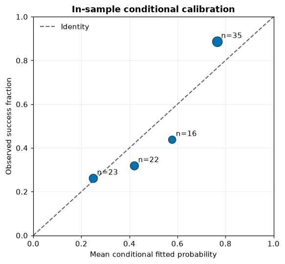
In-sample conditional calibration. Point size and labels communicate each bin’s sample size.

Interpretation. Points near the identity line indicate descriptive agreement on the analysis data. Because the lot modes were estimated from the same outcomes, this is a diagnostic view rather than out-of-lot validation.

2.12. Step 8: preserve approximation provenance

The manifest archives the Bernoulli model, data fingerprint, first-order Laplace method, reproducibility class, and optimizer sequence. The committed record identifies a deterministic-with-tolerance result and an optimizer sequence containing L-BFGS-B outer optimization, a Powell rescue, L-BFGS-B refinement, and BFGS conditional-mode optimization.

2.13. API map

Task	Public API
Select Bernoulli-logit	pymixef.families.Bernoulli
Declare the GLMM	pymixef.model.Model.from_formula()
Preview model compatibility	pymixef.model.Model.explain()
Compile and audit	pymixef.model.Model.compile(), pymixef.model.ExecutionPlan.explain()
Fit the Laplace model	pymixef.model.ExecutionPlan.fit()
Read estimates	pymixef.results.FitResult.parameters
Inspect approximation metadata	pymixef.results.FitResult.extra
Inspect outer and inner convergence	pymixef.results.FitResult.convergence
Read lot conditional modes	pymixef.results.FitResult.random_effects
Read conditional fitted probabilities	pymixef.results.FitResult.fitted_values
Inspect provenance	pymixef.results.FitResult.manifest, pymixef.provenance.RunManifest.to_dict()

Interpretation boundaries

The demonstrated path deliberately stays within the supported Bernoulli-logit, first-order Laplace calculation. It is most useful when the binary endpoint is scientifically meaningful and lot clustering is part of the design. When continuous response information is available, retain it where appropriate; when decisions must generalize to new lots, add held-out lot validation and sensitivity to approximation and random-effect assumptions. Keep odds ratios, conditional probabilities, marginalized probabilities, and validation targets explicitly labeled.

2.14. Exercises

1. Change the promoter generating effect from 0.45 to 0.0. How often does a finite sample still produce a nonzero estimate?

2. Increase the lot-intercept SD and inspect shrinkage in lot modes.

3. Replace the binary endpoint with counts and use the supported Poisson family after deciding what the exposure means.

4. Hold out entire lots and compute genuinely out-of-lot predictive metrics.

5. Request an unsupported extension and inspect the typed refusal instead of attempting to bypass it.

2.15. Takeaways

• Match the response distribution to the scientific endpoint.

• Account for repeated runs from the same lot.

• Interpret log-odds and odds ratios on their proper scale.

• Check both outer and conditional-mode convergence.

• Separate conditional, marginal, in-sample, and out-of-sample claims.