8. Closed-form pharmacokinetics and event-aware ODE simulation

Field: pharmacokinetics and clinical pharmacology
Analysis: one-compartment structural simulation
Calculation paths: closed form and event-aware ODE
Routes: IV bolus, finite IV infusion, and oral dosing

Download the complete, pre-executed notebook

8.1. Domain and problem

Pharmacokinetic models can often be evaluated in more than one way. A linear one-compartment IV-bolus model has a closed-form concentration function, while the same scientific model can be represented as a differential equation with a discontinuous dose event. Agreement between these paths is a valuable implementation cross-check.

This tutorial calculates both paths, requests a clearance sensitivity, compares input routes, and evaluates a combined additive-plus-proportional observation error model.

For dose \(D\), clearance \(CL\), and volume \(V\), the IV-bolus model is

\[ \frac{dA(t)}{dt}=-\frac{CL}{V}A(t),\qquad A(0^+)=D,\qquad C(t)=\frac{A(t)}{V}=\frac{D}{V}\exp\left(-\frac{CL}{V}t\right). \]

The analytic clearance sensitivity used to interpret the finite-difference output is

\[ \frac{\partial C(t)}{\partial CL} =-\frac{t}{V}C(t). \]

8.2. What you will learn

By the end of the tutorial, you will be able to:

1. evaluate supported one-compartment closed-form concentration functions;

2. represent central amount as an ODE state;

3. apply a bolus as an exact event-time discontinuity;

4. retrieve ODE state trajectories and solver metadata;

5. cross-check ODE and analytic concentration paths numerically;

6. request a finite-difference parameter sensitivity;

7. compare bolus, finite-infusion, and first-order oral input profiles; and

8. separate structural prediction from observation-error variance.

8.3. Dataset and model snapshot

This is a deterministic simulation rather than a fitted dataset.

Item	Value
Time grid	0 to 12 h in 0.5 h increments
Number of evaluation times	25
Dose	100
Clearance (CL)	5 L/h
Volume (V)	20 L
Elimination rate constant	0.25 h⁻¹
ODE state	Central amount
Reported structural output	Central amount / volume
Infusion duration	2 h
Oral absorption rate	1.2 h⁻¹
Additive error SD	0.10 mg/L
Proportional error SD	0.15

The implied IV-bolus concentration is

(dose / volume) * exp(-(clearance / volume) * time)

when amount, clearance, volume, and time use mutually consistent units.

8.4. Runnable core analysis

The following excerpt reproduces the analytic-versus-ODE comparison.

import numpy as np

from pymixef.pharmacometrics import (
    one_compartment_iv_bolus,
    simulate_ode,
)

times = np.linspace(0.0, 12.0, 25)
dose = 100.0
parameters = {"CL": 5.0, "V": 20.0}

closed_form = one_compartment_iv_bolus(
    times,
    dose=dose,
    clearance=parameters["CL"],
    volume=parameters["V"],
)

events = [
    {
        "ID": "S1",
        "TIME": 0.0,
        "EVID": 1,
        "AMT": dose,
        "CMT": "central",
    }
]


def elimination_rhs(time, state, context):
    del time
    rate_constant = context.parameters["CL"] / context.parameters["V"]
    return [-rate_constant * state[0]]


ode_result = simulate_ode(
    elimination_rhs,
    [0.0],
    events,
    t_eval=times,
    parameters=parameters,
    state_names=["central"],
    sensitivity_parameters=["CL"],
)
ode_concentration = ode_result.state("central") / parameters["V"]

maximum_difference = float(
    np.max(np.abs(ode_concentration - closed_form))
)
assert ode_result.metadata.success
assert maximum_difference < 1e-7

8.5. Step-by-step analysis

8.5.1. 1. Evaluate the closed-form IV-bolus model

one_compartment_iv_bolus(...) returns concentration values aligned to the requested time array.

The first six saved values are:

Time (h)	Concentration (mg/L)
0.0	5.000000
0.5	4.412485
1.0	3.894004
1.5	3.436446
2.0	3.032653
2.5	2.676307

At time zero, concentration is dose / volume = 100 / 20 = 5 mg/L.

8.5.2. 2. Represent the same science as an event-aware ODE

The ODE state is amount, not concentration:

dA/dt = -(CL / V) * A

The event manager adds 100 units to the central state at time zero. The right-hand-side callback reads parameters from context.parameters; it does not need to implement dose logic itself.

The saved solver metadata report:

• success: True;

• integration segments: 24;

• event actions: 1; and

• maximum absolute analytic-versus-ODE concentration difference: 2.3192008313799306e-09.

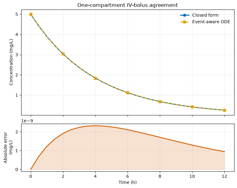
One-compartment IV-bolus agreement. The upper panel compares concentration curves; the lower panel exposes their absolute numerical difference.

Interpretation. The two concentration curves overlap at the plotted scale. The lower panel shows that the discrepancy remains below the asserted 1e-7 solver tolerance at every sampled time.

8.5.3. 3. Retrieve the clearance sensitivity

Because sensitivity_parameters=["CL"] was requested, the result contains the derivative of each state with respect to clearance.

amount_sensitivity_to_cl = ode_result.sensitivity("central", "CL")

The first eight saved values are:

Time (h)	dA/dCL
0.0	0.000000
0.5	-2.206242
1.0	-3.894004
1.5	-5.154670
2.0	-6.065307
2.5	-6.690768
3.0	-7.085498
3.5	-7.295085

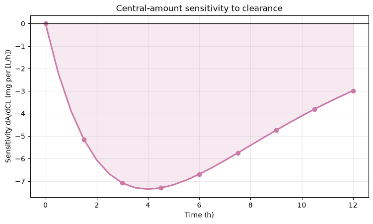
Central-amount sensitivity to clearance. The curve reports dA/dCL in amount per clearance units.

Interpretation. Sensitivity is zero at the instant of dosing and negative thereafter: increasing clearance reduces later central amount. Its changing magnitude shows when the trajectory is most responsive to a small clearance perturbation.

8.5.4. 4. Compare routes with the other parameters fixed

The package supplies closed-form helpers for a finite constant-rate infusion and first-order oral absorption.

from pymixef.pharmacometrics import (
    one_compartment_infusion,
    one_compartment_oral,
)

infusion = one_compartment_infusion(
    times,
    dose=100.0,
    duration=2.0,
    clearance=parameters["CL"],
    volume=parameters["V"],
)
oral = one_compartment_oral(
    times,
    dose=100.0,
    clearance=parameters["CL"],
    volume=parameters["V"],
    absorption_rate=1.2,
)

The saved peak summaries are:

Route	Peak concentration	Peak time on the grid
IV bolus	5.0	0 h
2 h IV infusion	3.9346934028736658	2 h
Oral, ka=1.2 h⁻¹	3.296781414122436	1.5 h

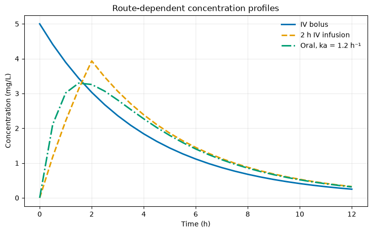
Route-dependent concentration profiles. Bolus, infusion, and oral input kinetics are compared under common clearance and volume.

Interpretation. The bolus produces an immediate peak, the finite infusion lowers and delays that peak, and first-order absorption shifts the oral maximum later. These differences arise from input kinetics because clearance and volume are held fixed.

8.5.5. 5. Evaluate declared observation-error variance

A combined error model adds an additive variance floor to a prediction-proportional component.

from pymixef.pharmacometrics import combined

observation_error = combined(
    additive_sigma=0.10,
    proportional_sigma=0.15,
)
variance = observation_error.variance(closed_form)

For this model,

variance(prediction) = 0.10² + (0.15 * prediction)²

The first six saved variances are:

Time (h)	Prediction (mg/L)	Variance ((mg/L)²)
0.0	5.000000	0.572500
0.5	4.412485	0.448075
1.0	3.894004	0.351173
1.5	3.436446	0.275706
2.0	3.032653	0.216932
2.5	2.676307	0.171159

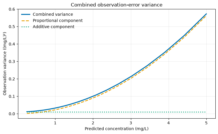
Combined observation-error variance. Total variance is decomposed into its additive and proportional components.

Interpretation. The proportional component grows quadratically with predicted concentration, while the additive component supplies a constant variance floor. The combined curve evaluates a declared measurement model; it does not estimate error parameters from these predictions.

8.6. Key saved results

Quantity	Saved value
Initial IV-bolus concentration	5.0 mg/L
Maximum ODE/closed-form difference	2.3192008313799306e-09 mg/L
Solver success	True
Solver segments	24
Event actions	1
Bolus peak	5.0 mg/L
Infusion peak	3.9346934028736658 mg/L
Oral peak	3.296781414122436 mg/L
Oral peak time on grid	1.5 h
Variance at 5 mg/L	0.5725 (mg/L)²

8.7. API map

Task	Public API	Result used here
IV-bolus closed form	pymixef.pharmacometrics.pk.one_compartment_iv_bolus()	Concentration array
Finite-infusion closed form	pymixef.pharmacometrics.pk.one_compartment_infusion()	Concentration array
First-order oral closed form	pymixef.pharmacometrics.pk.one_compartment_oral()	Concentration array
Event-aware integration	pymixef.pharmacometrics.ode.simulate_ode()	pymixef.pharmacometrics.ode.ODESimulationResult
Read parameters in RHS	pymixef.pharmacometrics.ode.ODEContext.parameters	Parameter mapping
Retrieve a state	pymixef.pharmacometrics.ode.ODESimulationResult.state()	Central-amount array
Retrieve sensitivity	pymixef.pharmacometrics.ode.ODESimulationResult.sensitivity()	\(dA/dCL\) array
Review solver work	pymixef.pharmacometrics.ode.ODESimulationResult.metadata	Solver metadata
Declare combined error	pymixef.pharmacometrics.pk.combined()	pymixef.pharmacometrics.pk.CombinedError
Evaluate error variance	pymixef.pharmacometrics.pk.CombinedError.variance()	Variance array

8.8. Exercises

1. Double clearance and explain the changes in half-life and exposure.

2. Add a second bolus event at 12 hours and extend t_eval to 24 hours.

3. Build an infusion event table and compare event-aware ODE output with one_compartment_infusion(...).

4. Move the oral absorption rate toward the elimination rate and inspect the helper’s stable limiting behavior.

5. Request a volume sensitivity and compare its sign and time profile with the clearance sensitivity.

Interpretation boundaries

Use this tutorial as a reproducible structural-model and numerical-consistency example. It simulates known individual parameters under linear one-compartment kinetics, assumes mutually consistent units, and uses finite-difference sensitivities. Agreement between two paths in the same package is strong regression evidence but is not independent external validation. For scientific inference, add parameter estimation, uncertainty, model selection, observation handling, and qualification appropriate to the data and intended decision.