4. Multicenter longitudinal biomarker with an LMM

This tutorial analyzes a continuous biomarker measured repeatedly within patients enrolled at multiple centers. Separate center and patient random intercepts represent two clustering levels while baseline, treatment, week, and treatment-by-week effects describe the adjusted mean trajectory.

The dataset is deterministic and synthetic; it contains no patient information.

Download the executed notebook

4.1. What you will learn

You will learn to:

• construct a reproducible multicenter longitudinal dataset;

• encode center and patient intercept heterogeneity separately;

• compile and inspect a Gaussian mixed model before optimization;

• fit the model with REML through PyMixEF’s public API;

• interpret the treatment-by-week interaction and variance components;

• inspect fixed-effect intervals and residual diagnostics; and

• distinguish an educational reference calculation from causal or confirmatory clinical evidence.

4.2. Domain question

Six centers enroll six patients each. Every patient is measured at weeks 0, 4, 8, and 12. Treatment is assigned at the patient level, and baseline remains constant within patient. The model is:

\[ \text{biomarker} \sim \text{baseline}+\text{treatment}\times\text{week} +(1\mid\text{center})+(1\mid\text{patient}). \]

The treatment-by-week coefficient asks whether the average longitudinal slope differs between arms after adjustment for baseline. The center and patient random intercepts capture distinct sources of unexplained baseline-level heterogeneity.

4.3. Dataset snapshot

Property	Value
Rows	144
Centers	6
Patients	36
Visits per patient	4
Visit weeks	0, 4, 8, 12
Overall biomarker mean	16.165906806474677
Generating center SD	1.2
Generating patient SD	2.0
Generating measurement SD	1.0
Random seed	20260704

4.4. Reproduce the data

The following runnable excerpts are taken from the executed notebook.

import importlib
import logging

import numpy as np

import pymixef

# Keep a fresh-kernel run free of Matplotlib's one-time font-cache status message.
logging.getLogger("matplotlib.font_manager").setLevel(logging.ERROR)
plt = importlib.import_module("matplotlib.pyplot")

plt.style.use("tableau-colorblind10")

SEED = 20260704
rng = np.random.default_rng(SEED)

n_centers = 6
patients_per_center = 6
visit_weeks = np.array([0.0, 4.0, 8.0, 12.0])
n_patients = n_centers * patients_per_center

center_index = np.repeat(
    np.arange(n_centers), patients_per_center * len(visit_weeks)
)
patient_index = np.repeat(np.arange(n_patients), len(visit_weeks))
week = np.tile(visit_weeks, n_patients)
treatment_by_patient = np.tile(
    np.array([0, 1, 0, 1, 0, 1]), n_centers
)
treatment = np.repeat(treatment_by_patient, len(visit_weeks))
baseline_by_patient = rng.normal(50.0, 7.0, n_patients)
baseline = np.repeat(baseline_by_patient, len(visit_weeks))

center_effect = rng.normal(0.0, 1.2, n_centers)
patient_effect = rng.normal(0.0, 2.0, n_patients)
measurement_error = rng.normal(0.0, 1.0, len(week))

biomarker = (
    8.0
    + 0.12 * baseline
    + 0.15 * week
    + 1.00 * treatment
    + 0.18 * treatment * week
    + center_effect[center_index]
    + patient_effect[patient_index]
    + measurement_error
)

data = {
    "biomarker": biomarker,
    "baseline": baseline,
    "week": week,
    "treatment": treatment,
    "center": np.array([f"C{i + 1}" for i in center_index]),
    "patient": np.array([f"P{i + 1:03d}" for i in patient_index]),
}

4.5. Step 1: begin with observed trajectories

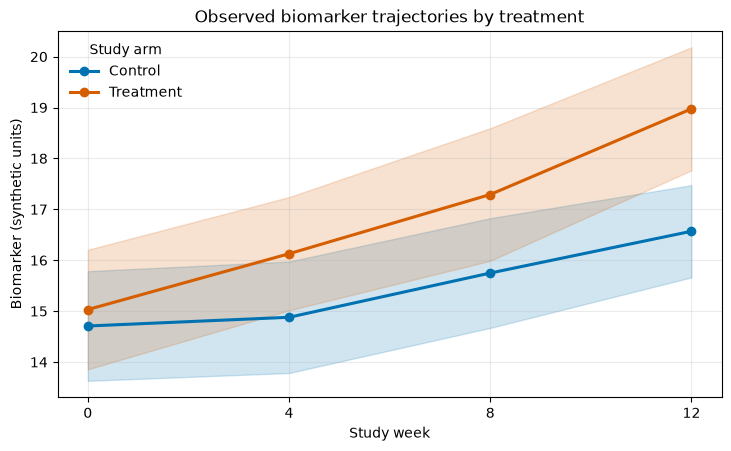
Observed biomarker trajectories by treatment.

Interpretation. Both arms rise over time, with visibly faster growth in the treated arm. These bands summarize raw means. The mixed model adds baseline adjustment and separates center, patient, and residual variation.

4.6. Step 2: declare and compile the model

Compilation constructs the fixed and random design matrices, audits input rows, resolves compatibility, and records semantic ModelIR before fitting.

model = pymixef.Model.from_formula(
    "biomarker ~ baseline + treatment * week + (1 | center) + (1 | patient)"
)
plan = model.compile(
    data,
    engine="lmm",
    method="reml",
    maxiter=400,
    compute_hessian=False,
)
print(plan.explain())

The committed plan contains a 144-by-5 fixed design of full rank. It has one random-intercept block for six centers, a second for 36 patients, and no excluded rows.

compute_hessian=False keeps the tutorial quick. The fit still archives the fixed-effect covariance used for the compact Wald display, but the notebook does not claim a complete Hessian-based uncertainty analysis.

4.7. Step 3: fit and check convergence

fit = plan.fit()
assert fit.convergence.trustworthy, fit.convergence.to_dict()
print(fit.summary())
print("\nConvergence trustworthy:", fit.convergence.trustworthy)
print("Manifest model hash:", fit.manifest.model_ir_hash)

The saved result converges trustworthily. Its ModelIR hash is sha256:ea0b988c07ad2431aeda4f358e0aacaad9b22775c953c28e16398c81f8f1e616.

4.8. Step 4: separate fixed effects and variance components

fixed_names = ["Intercept", "baseline", "treatment", "week", "treatment:week"]
fixed_effects = {name: fit.parameters[name] for name in fixed_names}
variance_components = {
    name: value
    for name, value in fit.parameters.items()
    if name.startswith("sd(") or name == "residual_sd"
}
assert fixed_effects["treatment:week"] > 0

4.8.1. Key saved results

Quantity	Estimate
Intercept	11.697153
Baseline coefficient	0.053898
Treatment difference at week 0	0.618475
Control-arm weekly slope	0.161316
Treatment-minus-control weekly slope	0.163521
Center-intercept SD	1.284691
Patient-intercept SD	1.884896
Residual SD	1.008321
Objective	262.0969405
Log likelihood	-262.0969405

The treatment-arm fitted slope is the sum of week and treatment:week, approximately 0.324836 biomarker units per week. The interaction is positive, matching the direction built into the synthetic data.

4.9. Step 5: display adjusted effects and uncertainty

fixed_covariance = np.asarray(fit.extra["fixed_effect_covariance"])
forest_names = fixed_names[1:]
forest_estimates = np.asarray([fit.parameters[name] for name in forest_names])
forest_standard_errors = np.sqrt(np.diag(fixed_covariance))[1:]

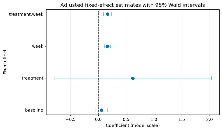
Adjusted fixed-effect estimates with 95% Wald intervals.

Interpretation. The positive treatment-by-week estimate supports the generated faster treated-arm slope. The interval display is useful for direction, magnitude, and precision in this synthetic fit; a confirmatory analysis would define its inferential method and targets in advance.

The intercept is omitted from the forest plot so the clinically interesting baseline, treatment, week, and interaction terms share a readable scale.

4.10. Step 6: inspect residual diagnostics

residual_table = fit.residual_diagnostics()
raw = residual_table.columns["raw_residual"]
{
    "rows": len(residual_table),
    "mean_residual": float(np.mean(raw)),
    "residual_rmse": float(np.sqrt(np.mean(raw**2))),
    "largest_absolute_residual": float(np.max(np.abs(raw))),
}

Residual diagnostic	Saved value
Rows	144
Mean raw residual	-1.603655480014115e-16
Residual RMSE	0.8730843233492872
Largest absolute residual	2.6632577080816127

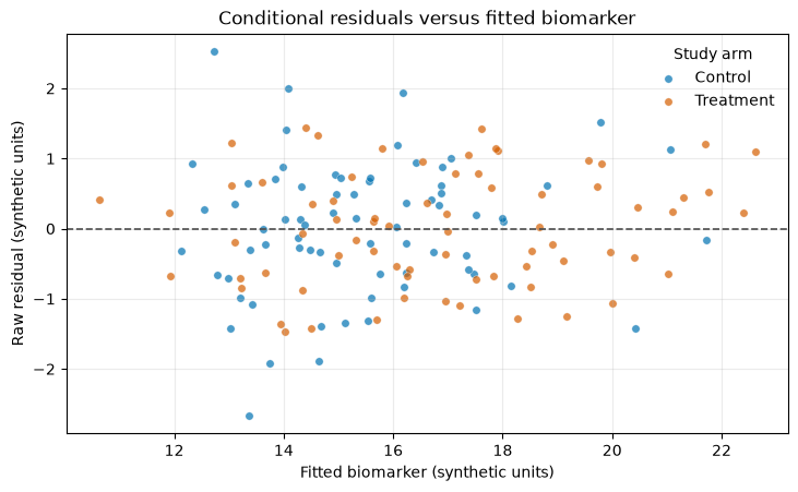
Conditional residuals versus fitted biomarker.

Interpretation. Residuals remain centered near zero across the fitted range, with broadly similar spread in the two arms. Reproducible curvature or widening would motivate revisiting the mean model or residual-variance assumptions.

4.11. API map

Task	Public API
Declare nested clustering	pymixef.model.Model.from_formula()
Compile and audit	pymixef.model.Model.compile(), pymixef.model.ExecutionPlan.explain()
Fit with REML	pymixef.model.ExecutionPlan.fit()
Check convergence	pymixef.results.FitResult.convergence
Print the fit	pymixef.results.FitResult.summary()
Read fixed and SD parameters	pymixef.results.FitResult.parameters
Read fixed-effect covariance	pymixef.results.FitResult.extra
Obtain conditional fitted values	pymixef.results.FitResult.fitted_values
Build a residual table	pymixef.results.FitResult.residual_diagnostics()
Read semantic provenance	pymixef.results.FitResult.manifest, pymixef.provenance.RunManifest.model_ir_hash

Interpretation boundaries

This synthetic study is designed to make two clustering levels and a treatment-by-time interaction easy to see. For causal, clinical, or regulatory questions, pair the same audited model workflow with the actual randomization and estimand, a prespecified uncertainty procedure, design-specific missing data and covariance reasoning, diagnostics, and independent validation. Turning off the optional numerical Hessian is appropriate for a quick walkthrough; analyses whose decisions depend on full uncertainty should enable and validate the intended inference path.

4.12. Exercises

1. Change the random seed and compare sampling variation in the interaction estimate.

2. Add a patient random slope with (1 + week | patient) and inspect the larger covariance block.

3. Introduce a few missing biomarker values and inspect the data audit in plan.explain().

4. Refit with method="ml" and explain why ML, rather than REML, is normally used for fixed-effect model comparisons.

4.13. Takeaways

• Center and patient random intercepts answer different clustering questions.

• The treatment-by-week interaction is the adjusted slope difference.

• Compile and audit before optimization.

• Inspect convergence separately from the parameter table.

• Use residual and uncertainty displays as diagnostics within a prespecified scientific analysis.